Tuesday B: Using UFO for bias correction and QC

1. Introduction

This practical session introduces the JEDI Unified Forward Operator (UFO) code and will teach you how to configure and run various bias correction and data quality control steps. The tutorial will begin with atmospheric motion vectors derived from infrared satellite data tracking of cloud motions. We will show a series of QC filter steps with these data. Then, we will show an example of bias correction of microwave satellite radiance data from SSMIS. Finally we will demonstrate quality control of infrared SEVIRI satellite data.

This activity assumes that you have successfully completed Monday’s activities. You should have a working build of the fv3-jedi bundle. You also should have access to the same academy node as before, either using the JupyterLab environment (recommended) or SSH.

Access your AWS instance and enter the Singularity container

Connect to your assigned compute node. You will use the same method as previous exercises.

You already have the singularity container that contains the JEDI dependencies. Enter the container using:

cd ~/
singularity shell -e jedi-gnu-openmpi-dev_latest.sif

Once in the container be sure also to remove limits the stack memory to prevent spurious failures as noted in yesterday’s introductory exercise.

ulimit -s unlimited
ulimit -v unlimited

2. Review of YAML structure

By now, you should have seen and experienced the structure of YAML files, so please refer to prior exercises of the Academy if editing of these files is not yet clear.

See this link for more examples.

3. Download and explore the test data

During the previous tutorial (#3), sample data were downloaded from our AWS data repository. So rather than re-download, we can explore the data again as a reminder.

cd ~/jedi/tutorials/tutorial_obs_data

The tutorial_obs_data directory contains excerpts of data generated from previous HofX model runs. Our radiance data are from a November 1, 2020, 12Z model run, and our conventional data are from December 15, 2020, 00Z. There are five subdirectories here, crtm, geoval, obs, aux_files, and answers.

• The obs subdirectory contains radiance observations from various instruments, including satellite platforms of AMSU-A, ATMS and SSMIS. There is also a variety of non-radiance data that we refer to as “conventional data,” including aircraft, surface observations, radiosondes, and wind data derived from satellite-detected cloud motion. These observation files are stored in IODA’s internal file format. Observation files can range in size from a few kilobytes to many megabytes. Some files store only a few observations, while others may contain millions.

• The geoval directory contains model state information that has been interpolated to the observation locations. GeoVaLs are “Geophysical Values at Locations.” In an ordinary JEDI run, we generate our own GeoVaLs in memory by consulting the model, but to save time in this practical we prepopulate our data from a previous invocation of JEDI.

• The crtm directory contains CRTM coefficient data used by the radiative transfer model.

• The aux_files directory contains auxilliary files for satellite biases and lapse rate information.

• The answers directory contains “hints” in case you get stuck when writing your YAML files.

Our tutorial begins with the atmospheric motion vector (AMV) data, which are created by tracking cloud motions through time using satellites. These are frequently called “SatWinds” while another type of satellite-derived wind motion data uses a scatterometer instrument for detecting ocean wave movement are frequently called “ScatWinds.”

The Satwind observation file is obs/satwinds_obs_2020121500_m.nc and contains over 50K data points in a 6-h time window. This file is reduced from the full volume of global data by a factor of about 50. The corresponding GeoVaLs file is: geoval/satwinds_geoval_2020121500_m.nc.

In a later step of this tutorial, we will be using satellite radiance data in the microwave and infrared regions. The Special Sensor Microwave Imager (SSM/I) and the Special Sensor Microwave Imager Sounder (SSMIS) are satellite passive microwave radiometers. For more complete details, see this SSMI link.

The corresponding satellite observation and GeoVaLs files are

obs/ssmis_f17_obs_2020110112.nc4
obs/seviri_m11_obs_2020110112.nc4
geoval/ssmis_f17_geoval_2020110112.nc4
geoval/severi_m11_geoval_2020110112.nc4

4. Quality control of SatWinds data.

In this step, we will write a YAML file to run a set of filters that decide which data are rejected and which are retained in the data assimilation. In general SatWinds data are already relatively high quality, because it is a “data product” derived from visible and infrared satellite detection of moving clouds. The producers, such as NOAA-NESDIS, Japan Meteorological Agency, and Europe’s EU-MET have already applied many quality control procedures in contrast to some other measurements such as surface weather observations. Regardless, we will demonstrate some extra precautions needed to ensure the DA system does not try to number-crunch potentially bad data.

Since we would like to avoid modifying our testing data, first create a new directory for our experiment.

mkdir -p ~/tutorial_4_experiments
cd ~/tutorial_4_experiments

Now, create a new YAML file, and name it satwinds_gfs_qc.yaml.

Insert the text block below into the new YAML file. In a YAML file, indentation is important, so please ensure that your file looks like this example. Also please ensure that your indents use spaces instead of tabs. If you are using the vi editor, it may be helpful to open the editor and immediately type :set paste so the indentation shown below should be kept the same.

window begin: 2020-12-14T20:30:00Z
window end: 2020-12-15T03:30:00Z

observations:
- obs space:
    name: satwinds_QC
    obsdatain:
      obsfile: /home/ubuntu/jedi/tutorials/tutorial_obs_data/obs/satwind_obs_2020121500_m.nc
    obsdataout:
      obsfile: /home/ubuntu/tutorial_4_experiments/satwind_obs_2020121500_m_out.nc
    simulated variables: [eastward_wind, northward_wind]
  geovals:
    filename: /home/ubuntu/jedi/tutorials/tutorial_obs_data/geoval/satwind_geoval_2020121500_m.nc
  obs filters:
#
# Before filtering any observations, there are 5247 missing U,V wind components out of the total 51007 obs,
# passedBenchmark: 91520 = 51007 x 2 (wind components) - 5247 missing of each component.
#
# Observation Range Sanity Check: either wind component or velocity exceeds 135 m/s
  - filter: Bounds Check
    filter variables:
    - name: eastward_wind
    - name: northward_wind
    minvalue: -135
    maxvalue: 135
    action:
      name: reject
  - filter: Bounds Check
    filter variables:
    - name: eastward_wind
    - name: northward_wind
    test variables:
    - name: Velocity@ObsFunction
    maxvalue: 135.0
    action:
      name: reject
#
# No observations exceed this threshold, but it is good as an absolute sanity check.
#
# Reject winds that are within 100 hPa of the surface.
  - filter: Difference Check
    filter variables:
    - name: eastward_wind
    - name: northward_wind
    reference: surface_pressure@GeoVaLs
    value: air_pressure@MetaData
    maxvalue: -10000
#
# The filter above rejects 4335 observed SatWinds.
#
# Reject winds that could be in the stratosphere (no clouds to track motion).
  - filter: Difference Check
    filter variables:
    - name: eastward_wind
    - name: northward_wind
    reference: TropopauseEstimate@ObsFunction
    value: air_pressure@MetaData
    minvalue: -3000                    # 30 hPa above tropopause level, negative p-diff
    action:
      name: reject
#
# The filter above rejects only 21 observed SatWinds.
#
# Reject when (O-B) difference of wind direction is more than 50 degrees, but only winds > 3 m/s.
  - filter: Bounds Check
    filter variables:
    - name: eastward_wind
    - name: northward_wind
    test variables:
    - name: WindDirAngleDiff@ObsFunction
      options:
        minimum_uv: 3.0
        test_hofx: GsiHofX
    maxvalue: 50.0
    action:
      name: reject
#
# The filter above rejects 3054 observed SatWinds.
#
# Perform special log-normal vector difference (LNVD), reject if larger than 3.
  - filter: Bounds Check
    filter variables:
    - name: eastward_wind
    - name: northward_wind
    test variables:
    - name: SatWindsLNVDCheck@ObsFunction
      options:
        testHofX: GsiHofX
    maxvalue: 3
    action:
      name: reject
#
# The filter above does not reject any of the observations.
#
# EUMET (242) and JMA (243) vis, reject when pressure less than 700 mb.
  - filter: Bounds Check
    filter variables:
    - name: eastward_wind
    - name: northward_wind
    test variables:
    - name: air_pressure@MetaData
    minvalue: 70000
    where:
    - variable:
        name: eastward_wind@ObsType
      is_in: 242, 243
    action:
      name: reject
#
# The filter above reject 237 observations.
#
# When running test_ObsFilters.x, We must tell the application how many observations
# remain after running all filters in each obs space.
  passedBenchmark: 76458

The different keys and groupings in the YAML file have meaning.

• The first two lines, window begin and window end, tell IODA the bounds of your assimilation window. All observations prior to and including the begin time or after the end time are dropped, i.e., (begin, end].

• The observations line and subsequent obs space start a new block in which input and output files are named. In contrast to the previous tutorial, we are not running an obs operator, HofX. Instead we will utilize the existing GeoVaLs file in which vertical columns of model data at observation points are already present. The advantage here is that we can develop UFO codes for filtering and QC of data in development mode to test various QC steps without the cost overhead of repeatedly running the HofX application.

• The obs filters section contains a lengthy set of filter steps, some are quite simple like Bounds Check and Difference Check, while a few require very specialized code called ObsFunctions to compute additional variables needed to test data quality. One example is the Difference Check to reject any SatWinds data that could possibly be in the stratosphere. This requires the special ObsFunction called TropopauseEstimate to find the approximate pressure of the tropopause in order to reject winds that might be more than a specified pressure lower (height higher) than the tropopause pressure (height). The filter found last in the YAML shows a powerful example of a where clause in which we are specifically targeting SatWinds from JMA or EU-Met to reject any data higher in the atmosphere than 700 hPa through the use of ObsType which is a 3-digit value associated with each instrument type that NCEP-EMC uses to identify many forms of data.

It must be noted that the order of filters in the YAML does not matter. For parallel computing reasons, the filters listed are not sequential and currently one filter does not depend on another. However, since a chain of filters can sometimes be very helpful, a future release of JEDI-UFO will include ability for users to list a dependency chain within the YAML.

6. Run the test application

The test application is named test_ObsFilters.x. It takes one command-line argument: the path to your YAML file. You could run the application directly, but you are processing many SatWinds observations. These can be parallelized by running within an MPI environment.

You can execute the program by typing this:

mpiexec -n 4 ~/jedi/build/bin/test_ObsFilters.x ~/tutorial_4_experiments/satwinds_gfs_qc.yaml

On the console you will notice a large amount of output. Eventually, the application should complete and return success, which is displayed on the second to final line with status = 0 displayed. If any errors are indicated that would be a status not equal zero, please ask for help to see what went wrong. Usually, there is a bad file path or a typo in the YAML.

You may need to scroll the output above many diagnostic print statements, but you can find out how many observations were either missing in the input data or filtered out by this YAML file by different filter groups. Try to locate the lines shown here:

QC satwinds_QC eastward_wind: 5247 missing values.
QC satwinds_QC eastward_wind: 3276 out of bounds.
QC satwinds_QC eastward_wind: 4255 rejected by difference check.
QC satwinds_QC eastward_wind: 38229 passed out of 51007 observations.
QC satwinds_QC northward_wind: 5247 missing values.
QC satwinds_QC northward_wind: 3276 out of bounds.
QC satwinds_QC northward_wind: 4255 rejected by difference check.
QC satwinds_QC northward_wind: 38229 passed out of 51007 observations.

Wind data are a bit unique compared to other observations, because you see a set of print statement for each wind component individually, which is why they look like duplicate prints. The prints are also aggregated for each filter type such as Bounds Check which was used 5 times in the YAML. Review the comments in the YAML below each filter to see the exact number of obs that would be eliminated if you had run that filter singularly in the YAML file.

Since we are running the test_ObsFilters.x application, we must supply the application with the final number of expected observations that successfully pass through the QC steps. So the last line of the YAML contains the key passedBenchmark to be considered a successful test. When running the JEDI software in regular mode of data assimilation, we will not know in advance the number of observations expected to pass, but this application would be substituted by another application in the regular execution of JEDI.

In our example dataset, roughly 25% of the starting observations are filtered by this QC yaml file.

7. Plotting the results

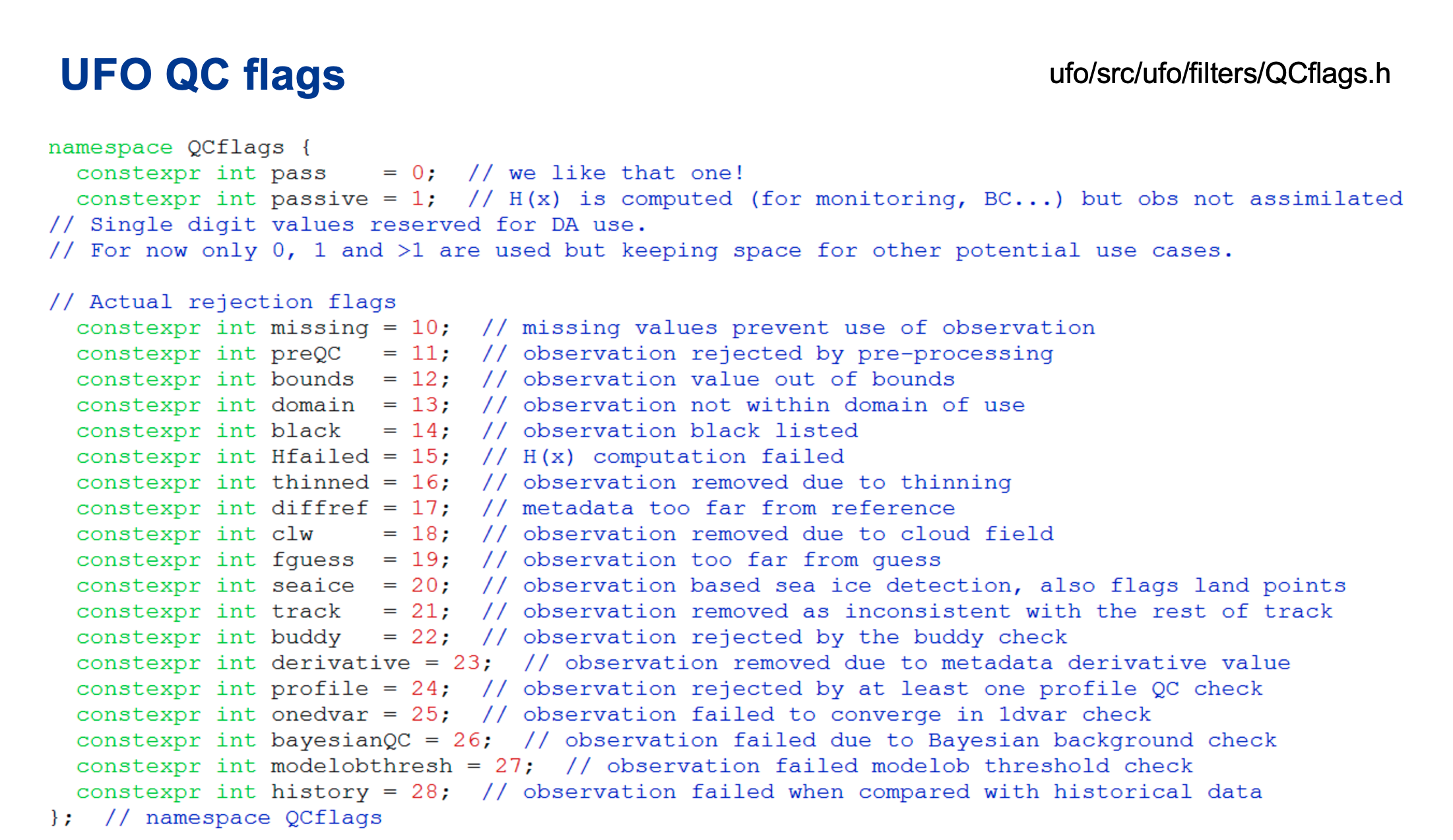
We can plot the observed wind components (eastward_wind, northward_wind) by running a python plotting script once for each variable. In addition, we can plot the results of our QC filter steps using the JEDI variable EffectiveQC which is a series of values to indicate which filter eliminated any observations. The source code file: ufo/src/ufo/filters/QCflags.h contains the integer value mapping of the filters shown in the image here:

Execute the plotting code for east/north winds and EffectiveQC using these commands:

python ~/jedi/tutorials/tutorial_obs_data/script/plot_from_iodav2_hofx.py --window_begin 2020121421 --nprocs 4 \
          --hofxfiles ~/tutorial_4_experiments/satwind_obs_2020121500_m_out_NPROC.nc \
          --colmin -45 --colmax 45 --variable ObsValue/eastward_wind
python ~/jedi/tutorials/tutorial_obs_data/script/plot_from_iodav2_hofx.py --window_begin 2020121421 --nprocs 4 \
          --hofxfiles ~/tutorial_4_experiments/satwind_obs_2020121500_m_out_NPROC.nc \
          --colmin -45 --colmax 45 --variable ObsValue/northward_wind
python ~/jedi/tutorials/tutorial_obs_data/script/plot_from_iodav2_hofx.py --window_begin 2020121421 --nprocs 4 \
          --hofxfiles ~/tutorial_4_experiments/satwind_obs_2020121500_m_out_NPROC.nc \
          --colmin -6 --colmax 12 --variable EffectiveQC/eastward_wind

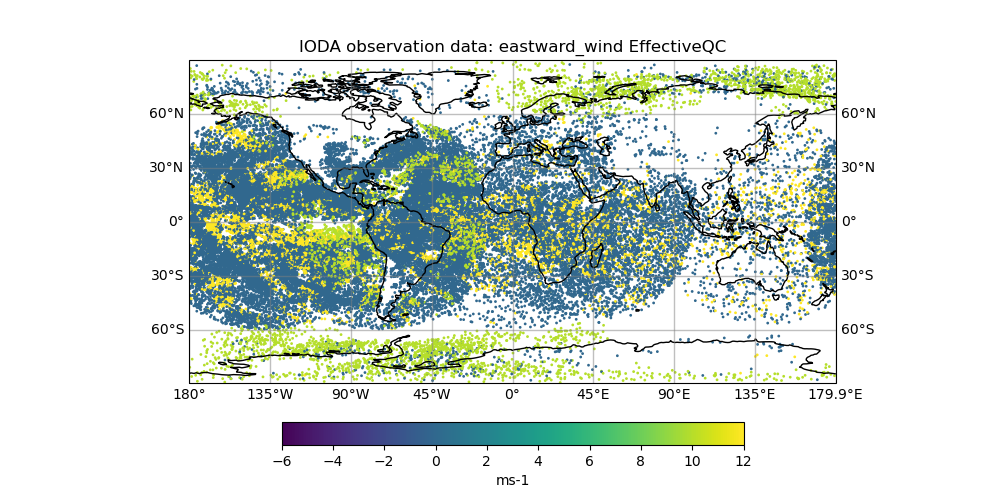
The graphics should look like the following example of eastward_wind observed values and the corresponding EffectiveQC 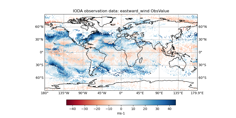and

The colorbars on the wind components are set to match between +-45 m/s for both wind components using the colmin and colmax command-line options for the observed wind values; otherwise the default plotting behavior assigns the colorbars based on the mean and standard deviation of the data. For the EffectiveQC plots, you can ignore the units label, because the color bar represents the integer of QC-flags shown above. The dots in blue shade all passed the QC, while the dots in green and yellow shades indicate QC flags that reject the data.

8. Create a YAML file to run the bias correction step for SSMIS satellite data.

We are now going to shift datasets entirely to show how UFO bias correction works with satellite radiance data from SSMIS.

We are going to write the YAML that specifies a number of predictors that modify the brightness temperature data in various channels to account for biases. Examples of the predictors are the sensor scan position and whether the satellite is in ascending or descending pass. There is a lecture tomorrow morning that clearly shows that some satellite channels are affected in systematic ways that can easily be adjusted by correcting for the bias. The changes you will make in this practical will illustrate how the data appear before and after the bias correction.

We should be certain that we are in the appropriate directory, so please execute:

cd ~/tutorial_4_experiments

Create a new YAML file, and name it ssmis_gfs_HofX_bc.yaml.

Insert this text into the new YAML file:

window begin: 2020-11-01T09:00:00Z
window end: 2020-11-01T15:00:00Z

observations:
- obs operator:
    name: CRTM
    Absorbers: [H2O,O3,CO2]
    obs options:
      Sensor_ID: &Sensor_ID ssmis_f17
      EndianType: little_endian
      CoefficientPath: /home/ubuntu/jedi/tutorials/tutorial_obs_data/crtm/
  obs space:
    name: ssmis_f17
    obsdatain:
      obsfile: /home/ubuntu/jedi/tutorials/tutorial_obs_data/obs/ssmis_f17_obs_2020110112.nc4
    obsdataout:
      obsfile: /home/ubuntu/tutorial_4_experiments/ssmis_f17_hofx_2020110112.nc4
    simulated variables: [brightness_temperature]
    channels: &channels 1-24
  geovals:
    filename: /home/ubuntu/jedi/tutorials/tutorial_obs_data/geoval/ssmis_f17_geoval_2020110112.nc4
  vector ref: GsiHofXBc
  tolerance: 1.e-5
  obs bias:
    input file: /home/ubuntu/jedi/tutorials/tutorial_obs_data/aux_files/satbias_ssmis_f17.nc4
    variational bc:
      predictors:
      - name: constant
      - name: cloud_liquid_water
        options:
          satellite: SSMIS
          ch19h: 12
          ch19v: 13
          ch22v: 14
          ch37h: 15
          ch37v: 16
          ch91v: 17
          ch91h: 18
      - name: cosine_of_latitude_times_orbit_node
      - name: sine_of_latitude
      - name: lapse_rate
        options:
          order: 2
          tlapse: &ssmis_f17_tlap /home/ubuntu/jedi/tutorials/tutorial_obs_data/aux_files/ssmis_f17_tlapmean.txt
      - name: lapse_rate
        options:
          tlapse: *ssmis_f17_tlap
      - name: emissivity
      - name: scan_angle
        options:
          var_name: scan_position
          order: 4
      - name: scan_angle
        options:
          var_name: scan_position
          order: 3
      - name: scan_angle
        options:
          var_name: scan_position
          order: 2
      - name: scan_angle
        options:
          var_name: scan_position

In a YAML file, indentation is important, so please ensure that your file looks like this example. Also please ensure that your indents use spaces instead of tabs. If you are using the vi editor, it may be helpful | to open the editor and immediately type :set paste so the indentation shown above should be kept the same.

The different keys and groupings in the YAML file have meaning.

• The first two lines, window begin and window end, tell IODA the bounds of your assimilation window.

• The observations line denotes that we are specifying an observation operator for the application to run. For this first example, we are only attempting to run a single observation operator, CRTM, as we used in a prior UFO practical. When CRTM performs its calculations, it will assume that the atmosphere has three absorbing gases, water vapor, ozone, and carbon dioxide. Water and ice clouds may both exist.

• The obs options section provides additional information to properly run CRTM. Each instrument needs various ancillary data files that contain information about the sensor’s channels, polarizations, spectral response funcitons, and so on.

• The obs space section describes the input data that we are using with the operator. The observation data file is specified using the obsfile key in the obsdatain section. The results of the operator can optionally be written to a file. This occurs when an obsdataout section appears in the YAML. The syntax of obsdatain and obsdataout are identical.

• The simulated variables and channels sections tell UFO that you want to simulate brightness temperatures for instrument channels 1-24.

• The geovals section provides interpolated model values at the observed locations. This is a “shortcut” for the JEDI system to avoid reading full model backgrounds, and this is very useful when developing a new operator or when incrementally implementing bias correction and quality control filters. For the purposes of this practical exercise (i.e. to keep runtimes short), we provide geovals files.

• The next two lines (vector ref and tolerance) allow us to specify a final “check” in our test application to verify that our simulated results match those of another system. In this case, we are matching against GSI’s H(x) operator and want to ensure that our calculations match theirs. If the reference check is not specified, then no check is performed.

• The obs bias section contains a variety of bias predictor names (to invoke functions) that are needed to calculate the bias correction to the microwave brightness temperature data.

References

Dee, D.P., 2004: Variational bias correction of radiance data in the ECMWF system. In Proc. ECMWF Workshop on Assimilation of High Spectral Resolution Sounders in NWP. ECMWF, Reading, UK, 97-112.

Zhu, Y., Derber, J., Collard, A., Dee, D., Treadon, R., Gayno, G., Jung, J.A., 2014. Enhanced radiance bias correction in the National Centers for Environmental Prediction’s Gridpoint Statistical Interpolation data assimilation system. Quarterly Journal of the Royal Meteorological Society 140, 1479–1492. https://doi.org/10.1002/qj.2233.

9. Run the test application

In a prior step, we only needed to run QC filters and not use any ObsOperator because we used pre-calculated GeoVaLs files. In this step, we will still run CRTM to simulate the satellite radiances, so we will use test application is named test_ObsOperator.x. It takes one command- line argument: the path to your YAML file. You could run the application directly, but you are processing many SSMIS observations. These can be parallelized by running within an MPI environment.

You can execute the program by typing this:

mpiexec -n 4 ~/jedi/build/bin/test_ObsOperator.x ~/tutorial_4_experiments/ssmis_gfs_HofX_bc.yaml

On the console you will notice a large amount of output. Eventually, the application should complete and return success, which is displayed on the second to final line with status = 0 displayed. If any errors are indicated that would be a status not equal zero, please ask for help to see what went wrong. Usually, there is a bad file path or a typo in the YAML.

10. Check the results

You may have noticed from the YAML defined and used in the previous sections that there was an obsdataout section in it. That section specifies an obsfile template name to save the output files of the run. So, let’s change the current directory to the one where those files are supposed to be saved and check them. On the console, you can change directory and list the files there:

You are expected to see a list of files similar to the following:

ssmis_gfs_HofX_bc.yaml
ssmis_f17_hofx_2020110112_0000.nc4
ssmis_f17_hofx_2020110112_0001.nc4
ssmis_f17_hofx_2020110112_0002.nc4
ssmis_f17_hofx_2020110112_0003.nc4

If you recall, the obsfile template was defined as /home/ubuntu/tutorial_4_experiments/ssmis_f17_hofx_2020110112.nc4 for this SSMIS case. The name of the files that you are seeing in your console follow that template, but you have four files following that template with an underscore and a set of numbers appended to its name (e.g., _0000). This is because you’ve run your application using four processor elements and the program distributes the input file among these four processor elements.

Let’s generate a figure showing some results from our run. To do this, we need to run the following command:

python ~/jedi/tutorials/tutorial_obs_data/script/plot_from_iodav2_hofx.py \
   --window_begin 2020110109 --nprocs 4 \
   --hofxfiles /home/ubuntu/tutorial_4_experiments/ssmis_f17_hofx_2020110112_NPROC.nc4 \
   --omb True \
   --variable hofx/brightness_temperature_24 --colmin -2 --colmax 2

The above command will invoke the plotting script passing a list of arguments, described as below:

• --window_begin 2020110109: the timestamp of the beginning of the window (following the YYYYMMDDHH template)

• --nprocs 4: number of processor elements used to run the application (same number of HofX files)

• --hofxfiles ../ssmis_f17_hofx_2020110112_NPROC.nc4: the template for HofX file names (with _NPROC appended to it)

• --omb True: we wish to plot the Obs minus background (O - B) data

• --variable hofx/brightness_temperature_24: the variable to be plotted (in this case the hofx of brightness_temperature for channel 24)

The command above is expected to generate a figure (brightness_temperature_24_omb.png) showing the spatial distribution of simulated brightness temperature observations minus background (from model using HofX) from SSMIS for channel 24 using all bias predictors to bias correct the observations.

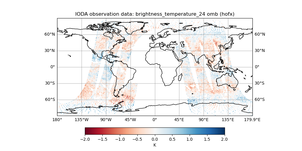
In the next section, we are going to remove all the sections in the YAML related to scan position to show the impact of skipping the bias correction for scan geometry. First, let’s be sure to save the first graphic we created in the example so far, so execute the follow command:

/bin/mv brightness_temperature_24_omb-hofx.png brightness_temperature_24_omb_step10.png

11. Remove the orbit node (ascending/descending) bias predictors

Edit the YAML file that we created in step#4 (ssmis_gfs_HofX_bc.yaml) and remove entirely the two lines shown below. This will eliminate the bias predictors related to whether the satellite is passing in ascending or descending modes, which have a known bias signal.

- name: cosine_of_latitude_times_orbit_node
- name: sine_of_latitude

Now we are going to re-run the same HofX and bias-correction HofX forward operator, except for skipping the two bias predictors. Recall the same execution command is this:

mpiexec -n 4 ~/jedi/build/bin/test_ObsOperator.x ~/tutorial_4_experiments/ssmis_gfs_HofX_bc.yaml

Due to removing two bias predictors, the number of observations that pass through the step changes, and we did not edit the number so an error message with non-zero status will occur. The step ran fine, so we will just ignore the error message.

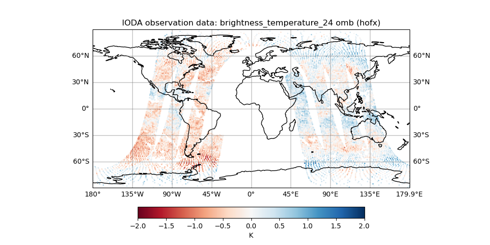
To visualize the result, we can re-create the same plot as the last time, but using the newly generated output (that overwrites the previous files) and shows what happens when we remove the bias predictor related to orbit node.

Re-run the plotting code again using:

python ~/jedi/tutorials/tutorial_obs_data/script/plot_from_iodav2_hofx.py \
   --window_begin 2020110109 --nprocs 4 \
   --hofxfiles /home/ubuntu/tutorial_4_experiments/ssmis_f17_hofx_2020110112_NPROC.nc4 \
   --omb True \
   --variable hofx/brightness_temperature_24 --colmin -2 --colmax 2

Now you can visually see the obs - background difference with and without accounting for bias correction of the satellite orbit node by comparing the two figures: brightness_temperature_24_omb_step10.png and brightness_temperature_24_omb.png.

12. Exercise: Add quality control for SEVIRI data and see its effect

For one final step, we will add quality control for SEVIRI data to eliminate any observations with local zenith angle greater than 50 degree. This is done due to the large slant angle through the atmosphere; only smaller zeninth angles are appropriate to ingest.

Create a new YAML file to quality control the SEVIRI satellite data, using the filename seviri_gfs_HofX_qc.yaml. Insert the following block of yaml into the new file.

window begin: 2020-11-01T09:00:00Z
window end: 2020-11-01T15:00:00Z

observations:
- obs operator:
    name: CRTM
    Absorbers: [H2O,O3,CO2]
    obs options:
      Sensor_ID: &Sensor_ID seviri_m11
      EndianType: little_endian
      CoefficientPath: /home/ubuntu/jedi/tutorials/tutorial_obs_data/crtm/
  obs space:
    name: seviri_m11_qc
    obsdatain:
      obsfile: /home/ubuntu/jedi/tutorials/tutorial_obs_data/obs/seviri_m11_obs_2020110112.nc4
    obsdataout:
      obsfile: /home/ubuntu/tutorial_4_experiments/seviri_m11_obs_2020110112_out.nc
    simulated variables: [brightness_temperature]
    channels: &all_channels 4-11
  geovals:
    filename: /home/ubuntu/jedi/tutorials/tutorial_obs_data/geoval/seviri_m11_geoval_2020110112.nc4
  obs filters:
#
# QC for local zenith angle ; only use data with less than 50 degree sensor zenith angle due to slant path potential problems.
  - filter: Domain Check
    filter variables:
    - name: brightness_temperature
      channels: *all_channels
    where:
    - variable:
        name: sensor_zenith_angle@MetaData
      maxvalue: 50.0
  passedBenchmark: 16444

Now we can run the QC steps using the test_ObsFilters.x application like we did for QC of Satwinds back in an earlier step using the following command line:

mpiexec -n 4 ~/jedi/build/bin/test_ObsFilters.x ~/tutorial_4_experiments/seviri_gfs_HofX_qc.yaml

This should result in four new output files (one file per core) for the SEVIRI output similar to a prior step for SSMIS output. Also, similar to the SatWinds QC example earlier, we can create a plot of the EffectiveQC performed by UFO using the command line:

python ~/jedi/tutorials/tutorial_obs_data/script/plot_from_iodav2_hofx.py --window_begin 2020110109 --nprocs 4 \
        --hofxfiles ~/tutorial_4_experiments/seviri_m11_obs_2020110112_out_NPROC.nc \
        --colmin 0 --colmax 19 --variable EffectiveQC/brightness_temperature_5

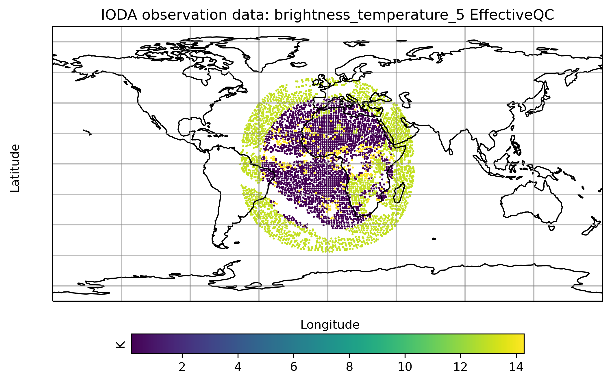
And, reaching the finish line for this tutorial, the result of the plot should look like the following image: