Wednesday A: Data Assimilation Diagnostics¶

In today’s tutorial we will build on the first steps taken earlier in the week and learn more about how to run the FV3-JEDI variational data assimilation application and how to modify it. First we will learn how to assess whether a particular run is healthy and then investigate some ways to change the run to improve the analysis.

In summary in this activity you will:

Learn how to check for healthy data assimilation runs in JEDI.

Get to know the variational data assimilation application.

Learn how to alter the behavior of the variation assimilation by adjusting the number of iterations.

Step 1: Download the data¶

In order to build on the work done previously we need some different data. This data will be the basis for this tutorial and the other tutorials covering FV3-JEDI over the week. Begin by downloading and extracting this data to your tutorials directory:

mkdir -p ~/jedi/tutorials
cd ~/jedi/tutorials
wget https://fv3-jedi-public.s3.amazonaws.com/Academy/1.1.0/20201001_0000z.tar
tar -xvf 20201001_0000z.tar

This directory contains everything needed to run a data assimilation application with JEDI. The files in this directory are designed to cover the 6 hour assimilation window that goes from 2020-09-30T21:00:00 to 2020-10-01T03:00:00. The name of the tar file and directory denotes the central time of the window. Take a minute to look around the 20201001_0000z/Data directory and familiarize yourself with the kinds of files that are required in order to run the data assimilation application. You’ll see background files through the window, ensemble files through the window for a 32 member ensemble, observations, CRTM coefficient files and some configuration files needed by FV3-JEDI. Today we will focus on the 3DEnVar assimilation run and so will use data valid at the center of the window, 2020-10-01T00:00:00

Step 2: Revive your environment¶

Before anything can be run we need to revive the parts of the environment that are not preserved when the instance is stopped and restarted.

Begin by entering the container again:

cd ~/
singularity shell -e jedi-gnu-openmpi-dev_latest.sif

Your prompt should now look something like:

Singularity>

Once in the container be sure also to remove limits the stack memory to prevent spurious failures:

ulimit -s unlimited
ulimit -v unlimited

FV3-JEDI-TOOLS was installed previously but the path still needs to be set in each session:

export PATH=$HOME/.local/bin:$PATH

Step 3: Rebuild JEDI in release mode¶

On Monday we built JEDI in a mode called RelWithDebInfo. This is often useful for development and for running the unit tests because it is faster than Debug mode but still contains trace information to help track and diagnose errors. But, the tutorials we will engage in today and tomorrow are more computationally expensive and we want the code to run faster.

So, let’s build again, this time in release mode. We’ll keep the old build around in case we have problems or in case you want to compare performance.

To build in release mode, enter the following commands

mkdir -p $HOME/jedi/build-release
cd $HOME/jedi/build-release
ecbuild --build=Release ../fv3-bundle
make -j8

The time it takes to build the code will be offset by the time you save running applications over the next few days.

Step 4: Run a 3DEnVar analysis for the C25 (4 degree model)¶

For simplicity make a convenience pointer to the place where the release version of JEDI is built:

JEDIBUILD=~/jedi/build-release/

Data assimilation involves a background error covariance model, which we will learn more about in the upcoming lectures on SABER and BUMP. The variational assimilation system we are running today uses a pure ensemble error covariance model but it requires localization in order to give a sensible analysis. The first step we need to take is to generate this localization model. Do not worry about understanding the configuration in this step, we will learn more about it later this week. To generate the localization model enter the following:

# Move to the directory where the executable must be run from
cd ~/jedi/tutorials/20201001_0000z

# Create a directory to hold the localization model files
mkdir -p Data/bump

# Run the application to generate the localization model
mpirun -np 6 $JEDIBUILD/bin/fv3jedi_parameters.x Config/localization_parameters_fixed.yaml

The localization model is fixed and does not even depend on the time for which the analysis is being run. So the above step is taken only once, even if changing the configuration for the variational assimilation.

Now we can run the data assimilation system and produce the analysis.

# Create directory to hold the resulting analysis
mkdir -p Data/analysis

# Create directory to hold resulting hofx data
mkdir -p Data/hofx

# Create directory to hold resulting log files
mkdir -p Logs

# Run the variational data assimilation application
mpirun -np 6 $JEDIBUILD/bin/fv3jedi_var.x Config/3denvar.yaml Logs/3denvar.log

Step 5: Check that we produced a healthy looking analysis¶

There are a number of diagnostics that can be useful for determining whether an assimilation run was healthy. That is to say whether the run has converged to within some criteria and produced a sensible analysis and fit to observations. The diagnostics we’ll explore in this tutorial are:

Plotting hofx [\(h({x})\)] and observation difference maps.

Plotting the convergence statistics.

Plotting the observation fit ‘innovation’ statistics.

Plotting the increment.

Configuration yaml files are provided to make plots for this experiment in the /Diagnostics directory.

First off we can generate the maps for the \(h({x})\) data using:

fv3jeditools.x 2020-10-01T00:00:00 Diagnostics/hofx_map.yaml

This will produce the hofx map plot for air temperature from the aircraft observations.

Note

This and other diagnostics will create a figure file. This file is located in a tutorials/20201001_0000z/Plots/ directory that will be created. The output path of the diagnostic can be adjusted in any of the configuration files in the Diagnostics/ directory.

You can try uncommenting and adjusting the values of colorbar minimum and colorbar maximum in the yaml file to produce a plot with better scaling. Note that you need to close the file before re-running, otherwise the file may not be overwritten. Now try adjusting the yaml to have metric: ombg and plotting again. You’ll need to choose the colorbar limit options in the configuration. This plot will show you the difference between the observation values and the background simulated observations [\(h({x_b})\)]. Now try plotting metric: oman, this will give you the difference between the observation values and the analysis simulated observations [\(h({x_a})\)]. You should notice some of the larger values disappear from the oman plot compared to the ombg plot. This is as expected, the analysis has moved the state closer to the observations.

You can also adjust the Diagnostics/hofx_map.yaml to plot the AMSUA data. Note that it is necessary to provide the channel number you wish to plot in addition to the field of brightness_temperature. Examples of this are commented out. You need to look at Config/3denvar.yaml to see which channels were actually assimilated.

That the assimilation draws closer to the observations can also be verified quantitiaively by examining the log file produced by the run. This file is located at Logs/3denvar.log. First of all you can search in this file for the string Jo/n. This will reveal lines like:

CostJo   : Nonlinear Jo(Aircraft) = 238308,      nobs = 268090, Jo/n = 0.88891,  err = 2.19395
CostJo   : Nonlinear Jo(AMSUA-NOAA19) = 52999.9, nobs = 60048,  Jo/n = 0.882626, err = 2.0023

In this example the value Jo/n = 0.88891 shows the fit to aircraft observations before the analysis and Jo/n = 0.882653 the fit to the AMSU-A observations before the analysis. By continuing to search through the file you will find values for Jo/n after the analysis. Here you’ll see lower values for each instrument, indicating a closer fit to the observations. Jo refers to the part of the cost function that measures the difference between the state and the observations. It is normalized by n, the number of observations.

The log file contains lots of other information about the convergence, but it is best to visualize this information to check the convergence, rather than looking through the log file. fv3-jedi-tools has the ability to create these diagnostics using the following:

fv3jeditools.x 2020-10-01T00:00:00 Diagnostics/da_convergence.yaml

This will produce five diagnostic plots showing aspects of the cost function. The key plot to look at is the one called drpcg-norm-reduction_20201001_000000.png. In a healthy data assimilation run the normalized gradient reduction will decline and then flatten off with some relatively small value. The plot produced should look similar to this:

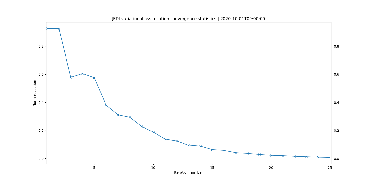
../../_images/drpcg-norm-reduction_20201001_000000.png

Initially the gradient reduction is a little erratic, but after 25 iterations or so the change from one iteration to the next is quite small, showing that the cost function is approaching its minimum, but perhaps not completely converged yet. Note that this metric is normalized with respect the the value at the beginning of the outer loop, so values are close to 1 at the beginning and then should reduce. In a typical operational weather forecast system values of the order of \(10^{-2}\) would be sufficient to indicate convergence. Though in most cases a maximum number of iterations would be satisfied before the value of the reduction.

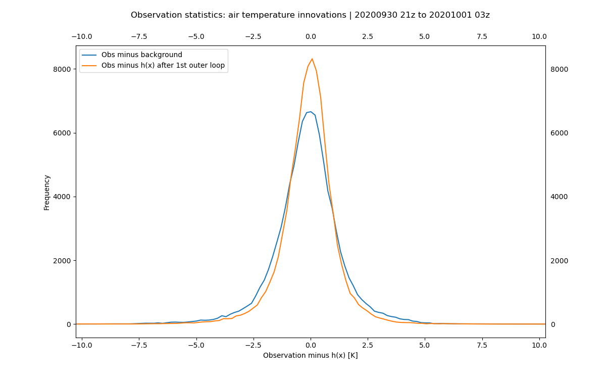
As mentioned above the assimilation should result in an analysis state closer to the observations than the background state was. While this is most readily verified by looking at the log, it is often useful to view this in a statistical sense as well. This can be done with the following:

fv3jeditools.x 2020-10-01T00:00:00 Diagnostics/hofx_innovations.yaml

The resulting plot (in Data/hofx/) should look similar to the below plot, with two probability distributions. In this figure the blue curve shows the probability for the observation minus observation simulated from the background and the orange curve the probability for the observation minus observation simulated from the analysis. The distribution has less spread and a mean closer to zero for the analysis. In Diagnostics/hofx_innovations.yaml there’s an option called number of bins, which determines the number of bins to use when creating the histograms, which are in turn interpolated to give the probability distributions. Try adjusting this number to see how the figure can change. If you decide to look at the AMSUA data you may need to use fewer bins to avoid noisy looking plots, you also need to request a certain channel number.

../../_images/air_temperature_innovations_20201001_000000.png

You can plot the increment produced by the assimilation. The first step is to generate the increment using the diffstates application as follows:

mkdir Data/increment
mpirun -np 6 $JEDIBUILD/bin/fv3jedi_diffstates.x Config/create_increment_3denvar.yaml

Once it has been created it can be plotted with:

fv3jeditools.x 2020-10-01T00:00:00 Diagnostics/field_plot.yaml

You can try adding more fields to the list and adjusting the level to be plotted in Diagnostics/field_plot.yaml. Note that you can do ncdump -h Data/increment/inc.3denvar.20201001_000000z.nc4 to see which fields are included in the analysis.

Step 6: Improve the analysis¶

Before continuing, make a backup of the data assimilation configuration file. In later tutorials we will use it as the starting point for other experiments.

cp Config/3denvar.yaml Config/3denvar_backup.yaml

If you open Config/3denvar.yaml you will see all the set up for the assimilation run. Scrolling to the bottom of this file you will find a section that looks like:

# Inner loop(s) configuration
variational:

  # Minimizer to employ
  minimizer:
    algorithm: DRPCG

  iterations:

  # First outer loop
  - ninner: 25
    gradient norm reduction: 1e-10
    test: on

    # Increment geometry
    geometry:
      trc_file: *trc
      akbk: *akbk
      layout: *layout
      io_layout: *io_layout
      npx: *npx
      npy: *npy
      npz: *npz
      ntiles: *ntiles
      fieldsets:
      - fieldset: Data/fieldsets/dynamics.yaml
      - fieldset: Data/fieldsets/ufo.yaml

    # Diagnistics to output
    diagnostics:
      departures: ombg

This part of the yaml controls the minimization of the cost function in the assimilation system. Variational data assimilation can consist of outer loops and inner loops. In the case show here one outer loop is used and there are 25 inner loops, denoted by the line ninner: 25. Inner loops essentially refer to the number of iterations taken to minimize the cost function. Between each outer loop the increment is added to the background and the cost function is re-linearized. As such a single outer loop with say 50 inner loops will produce a different result to using two outer loops with 25 inner loops each.

As we saw in some of the diagnostics above the assimilation system was not that well converged. Try adjusting to ninner: 100 in the yaml file. Then go back and run the assimilation again, the final part of Step 4: Run a 3DEnVar analysis for the C25 (4 degree model). With more inner loops now re-examine the diagnostics. How many inner loops is sufficient to see convergence? Note that running again as before will overwrite any previous diagnostics so you may wish to move them out of the way for comparison purposes.

Another thing that can be done is to add outer loops to the assimilation. There is no nouter in the configuration, this is controlled by inserting a list of outer loops in the yaml. Adding another outer loop in this example would look like:

# Inner loop(s) configuration
variational:

  # Minimizer to employ
  minimizer:
    algorithm: DRPCG

  iterations:

  # First outer loop
  - ninner: 25
    gradient norm reduction: 1e-10
    test: on

    geometry:
      trc_file: *trc
      akbk: *akbk
      layout: *layout
      io_layout: *io_layout
      npx: *npx
      npy: *npy
      npz: *npz
      ntiles: *ntiles
      fieldsets:
      - fieldset: Data/fieldsets/dynamics.yaml
      - fieldset: Data/fieldsets/ufo.yaml

    diagnostics:
      departures: ombg

  # Second outer loop
  - ninner: 25
    gradient norm reduction: 1e-10
    test: on

    geometry:
      trc_file: *trc
      akbk: *akbk
      layout: *layout
      io_layout: *io_layout
      npx: *npx
      npy: *npy
      npz: *npz
      ntiles: *ntiles
      fieldsets:
      - fieldset: Data/fieldsets/dynamics.yaml
      - fieldset: Data/fieldsets/ufo.yaml

    diagnostics:
      departures: ombg

Note that with two outer loops you need to adjust to number of outer loops: 2 in Diagnostics/hofx_innovations.yaml if using that diagnostic. Take a look through all the diagnostics. Did having a second outer loop help? Try playing with combinations of inner and outer loops and looking at how the results change.

Wednesday A: Data Assimilation Diagnostics¶

Step 1: Download the data¶

Step 2: Revive your environment¶

Step 3: Rebuild JEDI in release mode¶

Step 4: Run a 3DEnVar analysis for the C25 (4 degree model)¶

Step 5: Check that we produced a healthy looking analysis¶

Step 6: Improve the analysis¶

Table of Contents

Previous topic

Next topic

This Page