Tuesday A: Run H(x) in a testing environment

1. Introduction

This practical session introduces the JEDI Unified Forward Operator (UFO) code and will teach you how to configure and run a forward operator. You will then experiment with running operators on several radiance and conventional instruments. Finally, you will also make a few plots showing results.

This activity assumes that you have successfully completed Monday’s activities. You should have a working build of the fv3-jedi bundle. You also should have access to the same academy node as before, either using the JupyterLab environment (recommended) or SSH.

Access your AWS instance and enter the Singularity container

Connect to your assigned compute node. You will use the same method as yesterday.

You already have the singularity container that contains the JEDI dependencies. Enter the container using:

cd ~/
singularity shell -e jedi-gnu-openmpi-dev_latest.sif

Once in the container be sure also to remove limits the stack memory to prevent spurious failures as noted in yesterday’s introductory exercise.

ulimit -s unlimited
ulimit -v unlimited

2. Review of YAML structure

Programmers and computers typically store data as complex “objects” (structures and classes). In a computer’s memory, these objects may have very complicated storage involving pointers, references, dictionaries, and similar constructs. However, when we need to store these complex structures to a disk or send them across a network, we have to translate these complex structures into a series of bytes (a.k.a. we serialize an object into a byte stream).

There are many ways to do this. However, JEDI wanted to employ a consistent, well-documented format that is easy for people to edit and for machines to read. So, we chose to use the YAML Ain’t Markup Language (YAML) format to store the configuration data for the JEDI project.

YAML was developed in 2001 and has been implemented for use with several programming languages.

Let’s take a look at a YAML file for a brief overview.

---
# Comments are indicated with the '#' symbol.
name: "Your name here" # A string
a-boolean-value: true
an-integer-value: 3
pi: 3.14159
list-of-some-jedi-components:
  - saber
  - oops
  - ioda
  - ufo
dictionary-of-places-to-explore-in-a-staycation:
  - local-park:
    scenic: true
    features:
      - "Running trails"
      - Trees
      - "Duck pond"
  - aquarium:
    types-of-animals:
      - jellyfish
      - turtles
      - fish
      free: false
      mask: true
      # TODO: Explore this area and add more details.

The file starts with three dashes. These dashes indicate the start of a new YAML document. YAML supports multiple documents, and compliant parsers will recognize each set of dashes as the beginning of a new one.

Comments are started with a hashtag (“#”) and extend to the end of the line.

Next, we see the construct that makes up most of a typical YAML document: a key-value pair. “name” is a key that points to a string value: “Your name here”. YAML allows for several types of values: strings, integers, floating-point numbers, boolean values, and dates are all acceptable.

Strings can optionally be enclosed in quotes. Quotes include both single and double-quotes.

You can also add in arrays/lists. Each element in a list is denoted by an opening dash.

YAML elements can also be nested. This lets you emulate a group/folder structure. Nesting is accomplished by adding levels of spaces (no tabs allowed).

See this link for more examples.

3. Download and explore sample data

Sample data are available for download on our AWS data repository. Download these files into a dedicated test file directory. Untar the data archive and CD into it.

mkdir -p ~/jedi/tutorials
cd ~/jedi/tutorials
wget https://fv3-jedi-public.s3.amazonaws.com/Academy/1.1.0/tutorial_obs_data.tar
tar xf tutorial_obs_data.tar
cd tutorial_obs_data

The tutorial_obs_data directory contains excerpts of data generated from previous HofX model runs. Our radiance data are from a November 1, 2020, 12Z model run, and our conventional data are from December 15, 2020, 00Z. There are five subdirectories here, crtm, geoval, obs, answers, and aux_files.

• The obs subdirectory contains observations from various instruments, such as AMSU-A and ATMS. These observation files are stored in IODA’s internal file format. Observation files can range in size from a few kilobytes to many megabytes. Some files store only a few observations, while others may contain millions.

• The geoval directory contains model state information that has been interpolated to the observation locations. GeoVaLs are “Geophysical Values at Locations.” In an ordinary JEDI run, we generate our own GeoVaLs in memory by consulting the model, but to save time in this practical we prepopulate our data from a previous invocation of JEDI.

• The crtm directory contains CRTM coefficient data used by the radiative transfer model.

• The answers directory contains “hints” in case you get stuck when writing your YAML files.

• The aux_files directory contains auxilliary files for satellite biases and lapse rate information.

4. Create a YAML file to run the CRTM operator on AMSU-A data

We have a large number of observations available for radiance instruments. One of the most common instruments is AMSU-A, which has flown aboard the Aqua, MetOP-A, MetOP-B, MetOP-C, NOAA 15-19, NOAA 20, and Suomi-NPP satellites. Let’s consider MetOp-C, which launched in November 2018. The observation file is amsua_metop-c_obs_2020110112.nc4, and the GeoVaLs file is amsua_metop-c_geoval_2020110112.nc4.

We are going to write the YAML that instructs UFO’s H(x) testing application, test_ObsOperator.x, to read the testing file, run CRTM, and then store its simulated brightness temperatures. We will plot these simulated brightness temperatures and will also compare them against some data generated using NOAA’s Gridpoint Statistical Interpolation (GSI) system.

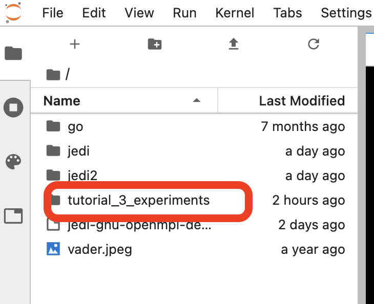
Since we would like to avoid modifying our testing data, first create a new directory for our experiment.

mkdir -p ~/tutorial_3_experiments
cd ~/tutorial_3_experiments

Create a new YAML file, and name it amsua_metop-c_gfs_HofX.yaml.

Insert this text into the new YAML file:

window begin: 2020-11-01T09:00:00Z
window end: 2020-11-01T15:00:00Z

observations:
- obs operator:
    name: CRTM
    Absorbers: [H2O,O3,CO2]
    Clouds: [Water, Ice]
    Cloud_Fraction: 1.0
    obs options:
      inspectProfile: 1
      Sensor_ID: amsua_metop-c
      EndianType: little_endian
      CoefficientPath: /home/ubuntu/jedi/tutorials/tutorial_obs_data/crtm/
  obs space:
    name: amsua_metop-c
    obsdatain:
      obsfile: /home/ubuntu/jedi/tutorials/tutorial_obs_data/obs/amsua_metop-c_obs_2020110112.nc4
    obsdataout:
      obsfile: /home/ubuntu/tutorial_3_experiments/out-amsua_metop-c_obs_2020110112.nc4
    simulated variables: [brightness_temperature]
    channels: 1-15
  geovals:
    filename: /home/ubuntu/jedi/tutorials/tutorial_obs_data/geoval/amsua_metop-c_geoval_2020110112.nc4
  vector ref: GsiHofX
  tolerance: 1.e-7

In a YAML file, indentation is important, so please ensure that your file looks like this example. Also please ensure that your indents use spaces instead of tabs.

The different keys and groupings in the YAML file have meaning.

• The first two lines, window begin and window end, tell IODA the bounds of your assimilation window. All observations outside of this window are dropped.

• The observations: line denotes that we are specifying a set of observation operators for the application to run. For this first example, we are only attempting to run a single observation operator. This operator is described on lines 5-14. We are invoking the CRTM operator. When CRTM performs its calculations, it will assume that the atmosphere has three absorbing gases, water vapor, ozone, and carbon dioxide. Water and ice clouds may both exist.

• The obs options section provides additional information to properly run CRTM. Each instrument needs various ancillary data files that contain information about the sensor’s channels, polarizations, spectral response funcitons, and so on. For AMSU-A on MetOp-C, the data are stored in a special Data/ directory. The amsua_metop-c files provide appropriate coefficients for our run. Note that occasionally there may be more than one set of available coefficients, and CRTM users are invited to read the CRTM documenation to determine which coefficients are appropriate.

• The obs space section describes the input data that we are using with the operator. The observation data file is specified using the obsfile key in the obsdatain section. The results of the operator can optionally be written to a file. This occurs when an obsdataout section appears in the YAML. The syntax of obsdatain and obsdataout are identical.

• The simulated variables and channels sections tell UFO that you want to simulate brightness temperatures for instrument channels 1-15.

• The geovals section provides interpolated model values at the observed locations. This is a “shortcut” for the JEDI system to avoid reading full model backgrounds, and this is very useful when developing a new operator or when incrementally implementing bias correction and quality control filters. For the purposes of this practical exercise (i.e. to keep runtimes short), we provide geovals files.

• The final two lines (vector ref and tolerance) allow us to specify a final “check” in our test application to verify that our simulated results match those of another system. In this case, we are matching against GSI’s H(x) operator and want to ensure that our CRTM calculations match theirs. If the reference check is not specified, then no check is performed.

5. Run the test application

The test application is named test_ObsOperator.x. It exists in your JEDI build directory (~/jedi/build/bin). It takes one command-line argument: the path to your YAML file. You could run the application directly, but you are processing many AMSU-A observations. These can be parallelized by running within an MPI environment.

You can execute the program by typing this:

mpiexec -n 4 ~/jedi/build/bin/test_ObsOperator.x ~/tutorial_3_experiments/amsua_metop-c_gfs_HofX.yaml

On the console you will notice a large amount of output. Eventually, the application should complete. If any errors are indicated (these are highlighted in red on the console), please ask for help to see what went wrong. Usually, there is a bad file path or a typo in the YAML.

6. Check the results

Checking among the diagnostic print statements, you can find out how different the UFO’s H(x) (hofx) is with respect to the reference set in the YAML, the GSI’s H(x) in this case (defined by vector ref: GsiHofX in the YAML above). Try to locate the line shown here:

Test     : Vector difference between reference and computed: amsua_metop-c nobs= 136095 Min=-4.49052e-05, Max=4.49696e-05, RMS=5.95927e-06

This line is presenting minimum, maximum and root mean squared differences between the simulated brightness temperature by UFO and GSI. The comparison is being performed considering all 15 channels together (remember that our YAML is set with channels: 1-15). This line is also presenting the number of observations (nobs). Considering the channels configuration and the number of observations, we can conclude that this test is being performed for 9073 locations with 15 channels each (\(9073 * 15 = 136095\)).

You may have noticed from the YAML defined and used in the previous sections that there was an obsdataout section in it. That section specifies an obsfile template name to save the output files of the run. So, let’s change the current directory to the one where those files are supposed to be saved and check them. On the console, you can change the directory and list the files there:

cd /home/ubuntu/tutorial_3_experiments
ls

You are expected to see a list of files similar to the following:

amsua_metop-c_gfs_HofX.yaml
out-amsua_metop-c_obs_2020110112_0000.nc4
out-amsua_metop-c_obs_2020110112_0001.nc4
out-amsua_metop-c_obs_2020110112_0002.nc4
out-amsua_metop-c_obs_2020110112_0003.nc4

If you recall, the obsfile template was defined as /home/ubuntu/tutorial_3_experiments/out-amsua_metop-c_obs_2020110112.nc4 for this amsua_metop-c case. The name of the files that you are seeing in your console follows that template, but you have four files following that template with an underscore and a set of numbers appended to its name (e.g., _0000). This is because you’ve run your application using four processor elements and the program distributes the input file among these four processor elements.

To avoid overwriting files, it’s important to create a folder to store the plots that will be drawn from the information inside these IODA files. You can do this on the console with the following commands:

mkdir amsua_metop-c
cd amsua_metop-c

Once inside the folder, let’s generate a figure showing some results from our run. To do this, we need to run the following command:

~/jedi/tutorials/tutorial_obs_data/script/plot_from_iodav2_hofx.py \
   --hofxfiles ../out-amsua_metop-c_obs_2020110112_NPROC.nc4 \
   --nprocs 4 \
   --window_begin 2020110109 \
   --variable hofx/brightness_temperature_10

The above command will invoke the plotting script passing a list of arguments, described as below:

• --hofxfiles ../out-amsua_metop-c_obs_2020110112_NPROC.nc4: the template for IODA file names (with _NPROC appended to it)

• --nprocs 4: number of processor elements used to run the application (same number of IODA files)

• --window_begin 2020110109: the timestamp of the beginning of the window (following the YYYYMMDDHH template)

• --variable hofx/brightness_temperature_10: the variable to be plotted (in this case the hofx of brightness_temperature for channel 10)

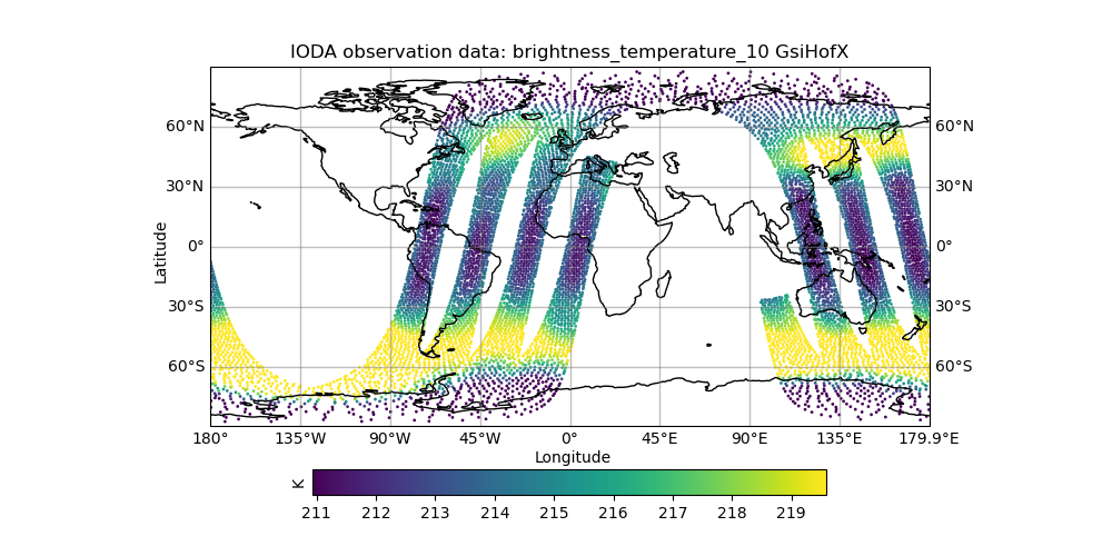
The command above is expected to generate a figure (brightness_temperature_10_GsiHofX.png) showing the spatial distribution of simulated brightness temperatures from amsua_metop-c for channel 10. You can view this figure in your JupyterLab environment by using the file explorer pane on the left side of your web browser window. Navigate to the /tutorial_3_experiments/amsua_metop-c directory in the file pane and you should be able to open and view the output plot.

Similarly, we can generate a figure showing the same quantity that has been generated previously by GSI. This quantity has been used previously as a reference in our test when running the application, and it’s stored in the IODA files named GsiHofX. To create the figure we need to run again the plotting script with slight different arguments:

~/jedi/tutorials/tutorial_obs_data/script/plot_from_iodav2_hofx.py \
   --hofxfiles ../out-amsua_metop-c_obs_2020110112_NPROC.nc4 \
   --nprocs 4 \
   --window_begin 2020110109 \
   --variable GsiHofX/brightness_temperature_10

To view this figure in JupyterLab, you may need to first refresh the file pane.

You may have noticed that in the above command we only changed the variables being plotted (from hofx/brightness_temperature_10 to GsiHofX/brightness_temperature_10). A first look into this newly generated figure for GSI reveals to be very similar to the previously generated for JEDI. They are qualitatively identical, but how different they are quantitatively? We can generate another figure presenting it using the following command:

~/jedi/tutorials/tutorial_obs_data/script/plot_from_iodav2_hofx.py \
   --hofxfiles ../out-amsua_metop-c_obs_2020110112_NPROC.nc4 \
   --nprocs 4 \
   --window_begin 2020110109 \
   --variable GsiHofX/brightness_temperature_10 \
   --jediminusgsi True

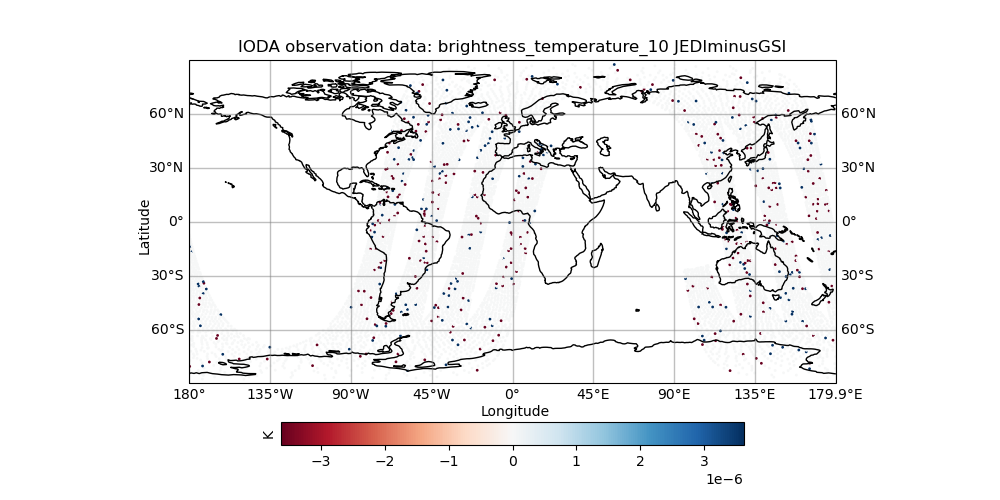
The above command is almost identical to the one that we’ve used to generate the figure for GSI, with the exception that an additional argument (--jediminusgsi True) has been passed to enable the plotting script to plot the difference between JEDI minus GSI for the simulated brightness temperature of channel 10. You can return to this section later and explore these plots for other channels if you have time.

7. Run the CRTM operator on ATMS data

The Advanced Technology Microwave Sounder (ATMS) instrument is a newer instrument that flies aboard Suomi-NPP and NOAA-20 (and eventually NOAA-21). ATMS combines the capabilities of both microwave temperature sounders (like AMSU-A) with microwave humidity sounders (MHS) into the same package. It has 22 channels from 23 GHz to 183 GHz.

Try going through the previous YAML configuration & program execution steps, but this time run the operator on ATMS data instead of AMSU-A data. You will need to:

• create a new YAML file / make a fresh copy of the AMSU-A file from before,

• update the CRTM YAML block to use ATMS coefficients,

• update the channel numbers,

• provide appropriate paths to the ATMS obs and geovals files, and

• specify a path for the output data.

Each of the files that you will need is in the same directories as their AMSU-A equivalents.

Run the test_ObsOperator.x application with your new YAML file. Have fun making plots of the output.

You can also experiment with plotting different channels.

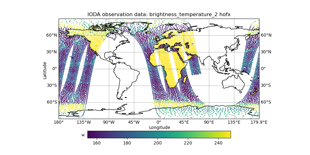
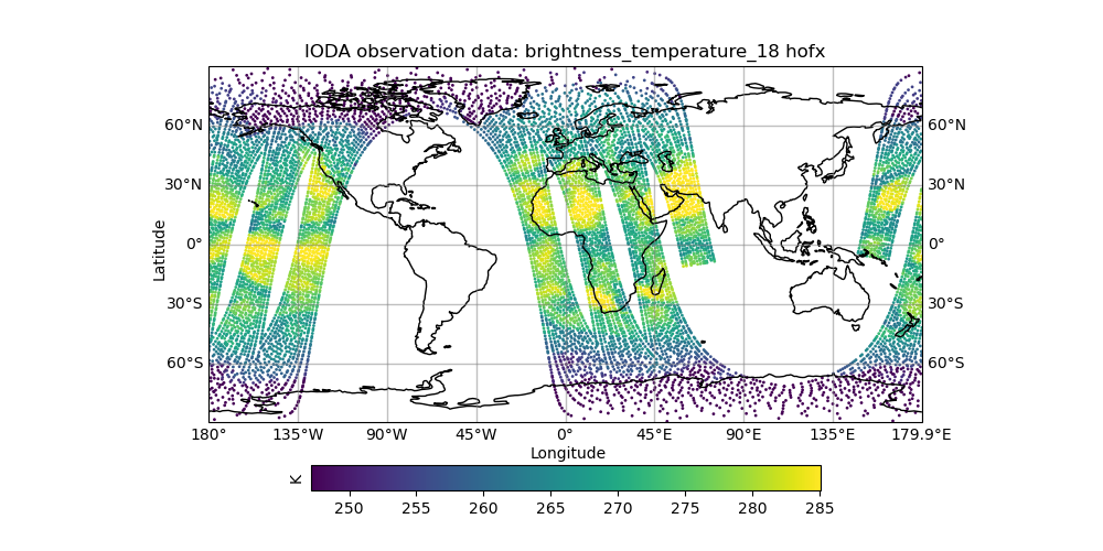
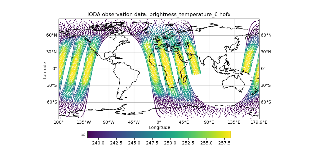
• Many of the lower ATMS channels are particularly good at detecting the Earth’s surface, and these channels show pronounced differences between land, ocean, and ice. [ Example image ]

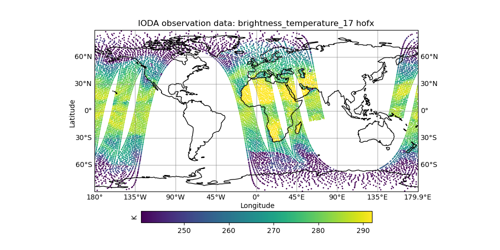
• ATMS channel 6 shows cross-swath bias effects. Bias correction will be discussed in this afternoon’s tutorial. [ Example image ]

• ATMS channels 17 and 18 (165.5 and 183.31 GHz, respectively) are particularly sensitive to clouds. [ Example image 1 ] [ Example image 2 ]

8. Run a conventional operator

There are many observation operators available within JEDI.

An important observation operator often used for conventional observations is the vertical interpolation operator. This operator is named inside UFO as VertInterp and it performs a linear vertical interpolation according to a given vertical coordinate. An example of its usage is when we want to simulate horizontal wind components obtained through satellites — the so-called satwinds. To be specific, these satwinds are referred to hereto as horizontal wind components obtained through the Atmospheric Motion Vectors (AMV) technique, which essentially derives these wind components identifying the movement of multiple patterns in a sequence of satellite images. It’s important to mention that this operator performs its vertical interpolation in logarithmic space when the vertical coordinate is pressure, which is the case for satellite winds here.

For a final exercise, try running the VertInterp operator on a small subset of our satwinds data.

Examine and use the following YAML. The obs operator section and simulated variables lines are subtly different from when we invoked CRTM, but the overall structure is the same.

window begin: 2020-12-14T21:00:00Z
window end: 2020-12-15T03:00:00Z

observations:
- obs operator:
    name: VertInterp
  obs space:
    name: Satwind
    obsdatain:
      obsfile: /home/ubuntu/jedi/tutorials/tutorial_obs_data/obs/satwind_obs_2020121500_m.nc
    obsdataout:
      obsfile: /home/ubuntu/tutorial_3_experiments/out-satwind_obs_2020121500_m.nc
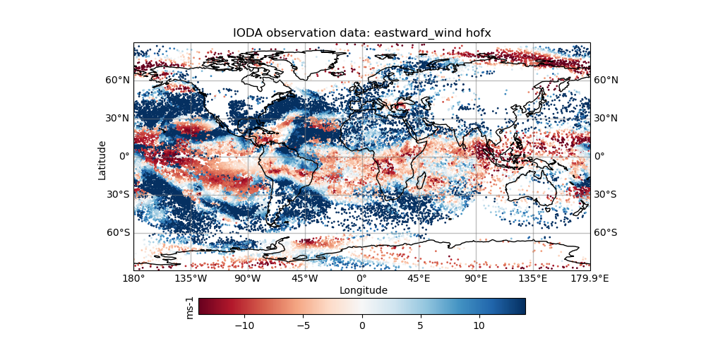
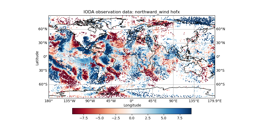
    simulated variables: [eastward_wind, northward_wind]
  geovals:
    filename: /home/ubuntu/jedi/tutorials/tutorial_obs_data/geoval/satwind_geoval_2020121500_m.nc
  vector ref: GsiHofX
  tolerance: 1.0e-02

After running the YAML, generate plots of the eastward_wind and northward_wind variables. You can also make plots of observations minus background (O-B). Note the colmin and colmax options: they set the range of the colorbar to sensible values.

mkdir -p ~/tutorial_3_experiments/satwind
cd ~/tutorial_3_experiments/satwind

~/jedi/tutorials/tutorial_obs_data/script/plot_from_iodav2_hofx.py --hofxfiles ../out-satwind_obs_2020121500_m_NPROC.nc --nprocs 4 --window_begin 2020121421 --colmin -45 --colmax 45 --variable hofx/northward_wind
~/jedi/tutorials/tutorial_obs_data/script/plot_from_iodav2_hofx.py --hofxfiles ../out-satwind_obs_2020121500_m_NPROC.nc --nprocs 4 --window_begin 2020121421 --colmin -45 --colmax 45 --variable hofx/eastward_wind

~/jedi/tutorials/tutorial_obs_data/script/plot_from_iodav2_hofx.py --hofxfiles ../out-satwind_obs_2020121500_m_NPROC.nc --nprocs 4 --window_begin 2020121421 --variable hofx/northward_wind --omb true
~/jedi/tutorials/tutorial_obs_data/script/plot_from_iodav2_hofx.py --hofxfiles ../out-satwind_obs_2020121500_m_NPROC.nc --nprocs 4 --window_begin 2020121421 --variable hofx/eastward_wind --omb true