Thursday A: Advanced model features
Note that tutorial “Data assimilation in 4D” is a prerequisite for this tutorial. You can obtain the solutions from these eariler tutorials by issueing:
wget https://fv3-jedi-public.s3.amazonaws.com/AcademyNov2020/Solutions4D.tar
In this tutorial we will explore some of the more advanced features of the assimilation runs as it relates to the model interface, these include:
Running with a pseudo model.
Running with lower resolution increments.
Running with dynamically generated B matrix models.
Step 1: Revive your environment
Before anything can be run we need to revive the parts of the environment that are not preserved when the instance is stopped and restarted.
Begin by entering the container again:
cd ~/
singularity shell -e jedi-gnu-openmpi-dev_latest.sif
Your prompt should now look something like:
Singularity>
Once in the container be sure also to remove limits the stack memory to prevent spurious failures:
ulimit -s unlimited
ulimit -v unlimited
If you didn’t already do this, you need to install the FV3-JEDI-TOOLS package to provide the diagnostics:
cd ~/jedi
git clone https://github.com/jcsda-internal/fv3-jedi-tools
cd fv3-jedi-tools
/usr/local/miniconda3/bin/pip install --user -e .
Even if FV3-JEDI-TOOLS was installed previously the path still needs to be set in each session:
export PATH=$HOME/.local/bin:$PATH
Set the path to the JEDI build directory
JEDIBUILD=~/jedi/build/
Step 2: Using a pseudo model and variables changes
So far we have been running 3DEVar-FGAT and 4DVar with the dynamical core model, which is a simplified version of the forecast model that does not have any physics. FV3-JEDI supports running with the full versions of GFS and GEOS but running those models is too expensive for a tutorial. When developing a new model interface for JEDI running with the full forecast model may not always be immediately available. There are often complexities with build systems and interfacing, especially if the models are not developed with being driven by the data assimilation in the scope of the design.
Alternatively its possible to use the so-called pseudo model, which just involves reading states from disk instead of running the forecast model. This separate executable mode would be more expensive but is useful for getting things running during development. OOPS provides an explicit “HofXNoModel.h” application, where a list of states is read in instead of reading the model for the \(h(x)\) calculation. Examples of this application are provided in the Ctests of the various models.
FV3-JEDI provides a pseudo model that can be used with the variational application. In this first part of the tutoriual we will learn how to run the 4DVar application with the Pseudo model. Begin by copying the 4DVar configuration from the earlier tutorial:
cd ~/jedi/tutorials/20201001_0000z
cp Config/4dvar.yaml Config/4dvar_pseudo.yaml
Note that if you added multiple outer loops to your 4DVar in the last practical you should revert to using a single outer loop. With the pseudo model it is not possible to run the forecast for the second outer loop in the same executable.
For the previous 4DVar run the forecast model part of the configuration looked like:
model:
  name: FV3LM
  nml_file: Data/fv3files/input_geos_c24.nml
  trc_file: Data/fv3files/field_table
  nml_file_pert: Data/fv3files/inputpert_4dvar.nml
  lm_do_dyn: 1
  lm_do_trb: 0
  lm_do_mst: 0
  tstep: PT1H
  model variables: [u,v,ua,va,t,delp,q,qi,ql,o3ppmv,phis,frocean,frlake,
                    frseaice,vtype,stype,vfrac,sheleg,ts,soilt,soilm,u10m,v10m]
To run with the Pseudo model change this to:
model:
  name: PSEUDO
  pseudo_type: geos
  datapath: Data/bkg
  filename_bkgd: geos.bkg.%yyyy%mm%dd_%hh%MM%ssz.nc4
  filename_crtm: geos.crtmsrf.c24.nc4
  run stage check: 1
  tstep: PT1H
  model variables: [u,v,ua,va,t,delp,q,qi,ql,o3ppmv,phis,
                    qls,qcn,cfcn,frocean,frland,varflt,ustar,bstar,
                    zpbl,cm,ct,cq,kcbl,tsm,khl,khu,frlake,frseaice,vtype,
                    stype,vfrac,sheleg,ts,soilt,soilm,u10m,v10m]
Note
Recall from the previous tutorials that when editing Yaml files the indent level is important. Use two spaces to indent directives that live within a particular section. Do not use tabs.
Note that the name of the model is now ‘PSEUDO’, telling the system to instantiate the pseudo model
object instead of the the FV3LM model. The only information the Pseudo model really needs is the path to
some files to read. It interprets the date time templates and reads the appropriate file for that
time step. In the directory Data/bkg you can see that files are available hourly, so the
time step is tstep: PT1H. Note that the list of variables has increased. Now that we have
the full forecast model (through files) we have some additional potential variables for the trajectory of the
tangent linear and adjoint version of the model.
As it stands these additional variables would also need to be added to the background configuration so that when the background is passed to the model it would have the correct variables. But this could lead to potential inefficiencies or complexities. For example if the model needs variables not available from the background directly. Instead we can use a variable change between the background and the model. FV3-JEDI and other models employ variable changes extensively to move between different parts of the cost function, where different variables are required. The below code shows how to add the variable change between the background and model. The other parts of the configuration are included to show the indent level required for the variable change.
background:
  filetype: geos
  datapath: Data/bkg
  filename_bkgd: geos.bkg.20200930_210000z.nc4
  filename_crtm: geos.crtmsrf.c24.nc4
  psinfile: true
  state variables: *anvars

# Variable change from background to model
variable change: Analysis2Model
filetype: geos
datapath: Data/bkg
filename_bkgd: geos.bkg.%yyyy%mm%dd_%hh%MM%ssz.nc4
filename_crtm: geos.crtmsrf.c24.nc4

model:
  name: PSEUDO
  ...
Note that we can now drastically reduce the number of variables in the background configuration,
so they contain only the variables necessary to create the increment. The more extensive list of
variables is restricted only to the model, which can save memory. The & and * are
special characters in Yaml files that eliminate the need to specify the same information more than
once. Therefore the anvars are just taken from where they are specified above.
Previously, when looking at diagnostics we examined \(h(x)\) for the background and analysis.
These statistics, including the Jo/n quantity, cannot be examined for the analysis in this
case because the forecast is not run for the analysis, the pseudo model can only read the same set
of files. We would have to run another forecast for the full model in another application. You can
still look at the convergence and increment at the beginning of the window though.
Before running, be sure to update the names of the analysis and \(h(x)\) output so as not to overwrite the previous 4DVar runs. Now you can run the pseudo model 4DVar:
mpirun -np 6 $JEDIBUILD/bin/fv3jedi_var.x Config/4dvar_pseudo.yaml Logs/4dvar_pseuso.log
Step 3: Running with different resolution increment
In practice variational data assimilation is performed with the increment at a lower resolution. This is often called incremental variational data assimilation. For algorithms such as 4DVar, the minimization step can be quite expensive since operators like the model adjoint and the B matrix have to be applied a large number of times. By running the minimization at lower resolution these costs can be reduced. Developing an operational data assimilation system is all about a balancing resolution, numbers of observations and complexity in the various operators to produce the most accurate analysis given the time constraints to deliver the forecast. Having the ability to run with low resolution increments is a very effective way to deliver a better analysis.
So far we have run all of the assimilation integrations with 25 grid points along each dimension of the cube face. This is controlled in the geometry part of the configuration file:
geometry:
  npx: &npx 25
  npy: &npy 25
Note that in some files this is referred to as “C24”, meaning 24 grid cells along each face of the
cube. This geometry lies in the cost function part of the configuration. Note that there is
another geometry section in the configuration which lies in the variational part of the
configuration. This horizontal resolution there is given as:
geometry:
  npx: *npx
  npy: *npy
Begin by creating a copy of the 4dvar_pseudo.yaml configuration file, that will be where we start from:
cp Config/4dvar_pseudo.yaml Config/4dvar_pseudo_lowresinc.yaml
In order to run with an increment with a different resolution to the background the geometry in the
variational part of the configuration needs to be changed. For this testing we will use
13 grid points along each dimension of the cube. The new geometry will be:
geometry:
  trc_file: *trc
  akbk: *akbk
  layout: *layout
  npx: 13
  npy: 13
  npz: *npz
  fieldsets:
  - fieldset: Data/fieldsets/dynamics.yaml
  - fieldset: Data/fieldsets/ufo.yaml
Only change the geometry in the variational part of the configuration, and not in the
cost function part. We do not want to change the resolution of the background.
For variational data assimilation the ensemble resolution needs to match the resolution of the
increment. Right now the ensemble resolution is with the 25 grid points. FV3-JEDI comes with an
application for changing the resolution of states. There exists a configuration file called
Config/change_resolution_ensemble.yaml for changing the resolution of the ensemble members
that are valid at the beginning of the window. Before running the low resolution 4DVar we need to
call the application to lower the resolution of the ensemble:
mpirun -np 6 $JEDIBUILD/bin/fv3jedi_convertstate.x Config/change_resolution_ensemble.yaml
There should now be files like Data/ens/*/geos.ens.c13.20200930_210000z.nc4 for each
member. Note that the output files have a slightly different name from before, to prevent them
being overwritten. This new name has to be taken into account in Config/4dvar_lowresinc.yaml.
Demonstrated for the first two members the configuration should look something like:
members:
  - filetype: geos
    state variables: *anvars
    datapath: Data/ens/mem001
    filename_bkgd: geos.ens.c13.20200930_210000z.nc4
    psinfile: true
  - filetype: geos
    state variables: *anvars
    datapath: Data/ens/mem002
    filename_bkgd: geos.ens.c13.20200930_210000z.nc4
    psinfile: true
Of course in practice the background and ensemble are typically already at different resolutions, the background being the resolution of the forecast model and the ensemble typically some lower resolution so as to afford the multiple required forecasts. Here we lower the resolution of the ensemble artificially to demonstrate and learn about this capability of the system.
Since the resolution of the ensemble has changed so must the localization model. This is achieved by
altering the geometry in the localization_parameters_fixed.yaml configuration. To be safe
first make a copy of that file:
cp Config/localization_parameters_fixed.yaml Config/localization_parameters_fixed_c13.yaml
Now open this file and edit the geometry part of the configuration in the same way that was done
in 4dvar_pseudo_lowresinc.yaml. Also change the name of the output files that will contain
localization model so as not to overwrite the higher resolution model. This can be done by appending
the prefix directive as follows:
bump:
  prefix: Data/bump/locparam_c13
Now you can create this new localization model:
mpirun -np 6 $JEDIBUILD/bin/fv3jedi_parameters.x Config/localization_parameters_fixed_c13.yaml
Since the name of the files containing the localization model has changed the corresponding update
needs to happen in Config/4dvar_pseudo_lowresinc.yaml. In the localization.bump part
of the config look for the prefix key and append it with c13 identially to how you did so in
Config/localization_parameters_fixed_c13.yaml.
The geometry of the actual linear model is not controlled through the main configuration file but
an underlying file that is read by the FV3 dynamical core. This file is located at
Data/fv3files/input_geos_c24.nml. First make a copy of this file called
Data/fv3files/input_geos_c12.nml and then edit npx and npy inside it. Find
the reference to Data/fv3files/input_geos_c24.nml in the linear model part of
Config/4dvar_lowresinc.yaml and update it to Data/fv3files/input_geos_c12.nml
Now you should be ready to run the low resolution 4dvar:
mpirun -np 6 $JEDIBUILD/bin/fv3jedi_var.x Config/4dvar_pseudo_lowresinc.yaml Logs/4dvar_pseuso_lowresinc.log
You may have already noticed that the run was faster than the previous 4DVar pseudo model run. One of the diagnostic utilities that we have not yet explored is to look at the timing of the runs. OOPS outputs extensive timing statistics and FV3-JEDI-TOOLS provides a mechanism for visualizing them.
You can generate the timing plots for the original pseudo model run with:
fv3jeditools.x 2020-10-01T00:00:00 Diagnostics/log_timing.yaml
To plot the timing diagnostics for the low resolution increment run edit Diagnostics/log_timing.yaml
to point to the that log file and rerun the above command.
The below figures show how the cost of the linear model changes as a percentage of the total cost
when changing to use a low resolution increment. The diagnostic also provides a file showing the
cost of methods per call to that method. The total cost is contained in files called e.g.
Logs/4dvar_pseuso_method_total_time_20201001_000000.png and the time used per call in files
like Logs/4dvar_pseuso_method_per_call_20201001_000000.png.
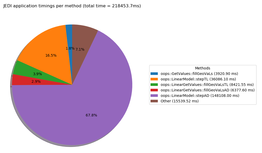
This figure shows the timing for the pseudo model run. The cost of running the model adjoint accounts for around 67% of the total run time.
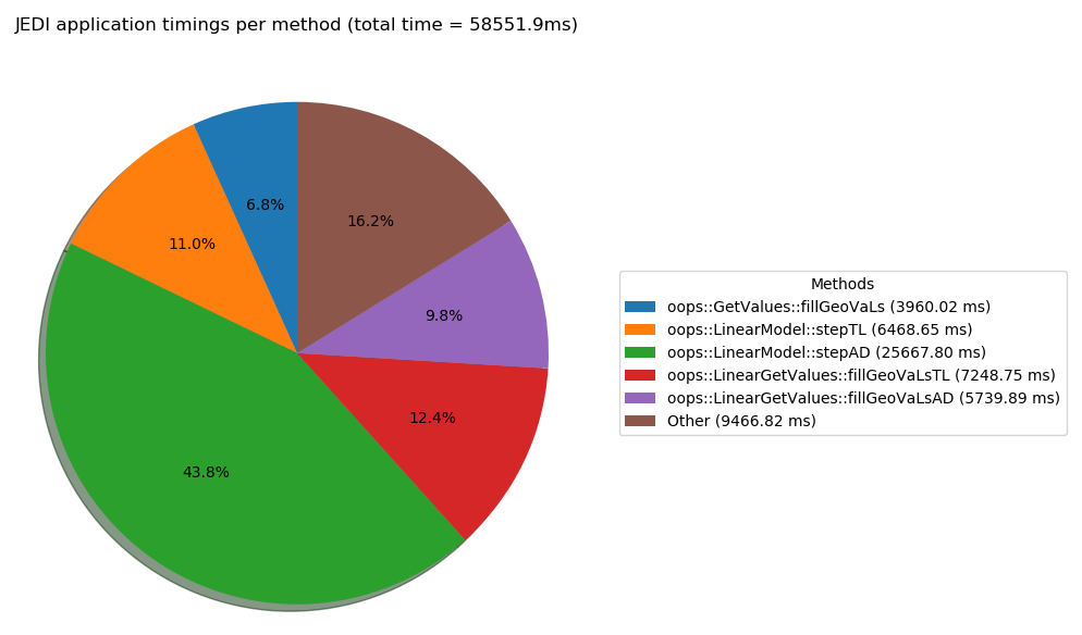
This figure shows the timing for the pseudo model with low resolution increment run. The cost of running the model adjoint accounts for around 44% of the total run time.
Step 4: Using localization length scales determined from the ensemble
The Config directory contains a configuration file for generating the localization model from the ensemble rather than using specified length scales. To invoke this method of generating the localization model enter:
mpirun -np 6 $JEDIBUILD/bin/fv3jedi_parameters.x Config/localization_parameters_dynamic.yaml
Note that this will take quite a bit longer to run than when generating a fixed scale localiztion
model. Once it completes additional files in the Data/bump directory called
Data/bump/locparam_dynamic_00_nicas_* should appear. To use this new localization model it
is necessary to update the variational configuration file. First make a copy:
cp Config/4dvar_pseudo.yaml Config/4dvar_pseudo_dynamicloc.yaml
Now you need to edit the localization part of the configuration to use the newly generated
model. The configuration should be:
bump:
  prefix: Data/bump/locparam_dynamic
  method: loc
  strategy: common
  load_nicas: 1
  mpicom: 2
  verbosity: main
Note that the io_key references can be removed now. These were used previously because variables
with different names would share a localization model. Try running this new case:
mpirun -np 6 $JEDIBUILD/bin/fv3jedi_var.x Config/4dvar_pseudo_dynamicloc.yaml Logs/4dvar_pseuso_dynamicloc.yaml
Try looking at some of the diagnostics for this run compared to the run with fixed localization length scales.