Tuesday B: Adding new observations to be assimilated

Introduction:

In this activity we will take a look at adding new observations into this mornings’s 3DVar exercise. This task typically involves the following steps:

1. Convert your raw observation file into a IODA formatted observation file.

2. Add a new ObsSpace definition to the YAML configuration file for the 3DVar run.

These tasks can involve some software development depending on whether your new observation type can be handled by existing IODA file converter programs and UFO obs operators. For today’s exercise, we will use existing IODA observation files and UFO obs operators, reducing your task to simply editing the 3DVar YAML configuration file.

The goal of this exercise is to learn how to manage the assimlation of different sets of observations in the JEDI system.

Step 1: Save results from this morning

We are going to add the new observation type, regenerate the results and then compare the new results to this mornings’s results. To get everyone on the same page, let’s rerun the original 3DVar assimilation from this morning’s exercise. This entails resetting the looping controls back to a single outer loop with 25 iterations of the inner loop.

Note

One option for editing is to click on the yaml file name in the JupyterLab directory listing on the left side. This brings up a native JupyterLab editor which includes decent yaml highlighting.

# Re-run original 3DVar assimilation
cd ~/jedi/tutorials/20201001_0000z

# Use your favorite editor to edit the configuration file
# Example below is for the 'vi' editor
vi Config/3denvar.yaml
  # Go to end of file in the "variational" section
  # Comment out any extra outer loop specifications
  # Make sure the single "- inner" spec is set to 25

The tail end of the Config/3denvar.yaml file should look like this:

# Inner loop(s) configuration
variational:

  # Minimizer to employ
  minimizer:
    algorithm: DRIPCG

  # First outer loop
  iterations:

  - ninner: 25
    gradient norm reduction: 1e-10
    test: on

    # Increment geometry
    geometry:
      trc_file: *trc
      akbk: *akbk
      layout: *layout
      npx: *npx
      npy: *npy
      npz: *npz
      fieldsets:
      - fieldset: Data/fieldsets/dynamics.yaml
      - fieldset: Data/fieldsets/ufo.yaml

    # Diagnistics to output
    diagnostics:
      departures: ombg

Re-run the assimilation:

cd ~/jedi/tutorials/20201001_0000z
JEDIBUILD=~/jedi/build

# run the 3DVar assimilation
mpirun -np 6 $JEDIBUILD/bin/fv3jedi_var.x Config/3denvar.yaml Logs/3denvar.log

# create the increment
mpirun -np 6 $JEDIBUILD/bin/fv3jedi_diffstates.x Config/create_increment_3denvar.yaml

There are a couple of plots that will be helpful for today’s exercise so let’s make sure these have been generated.

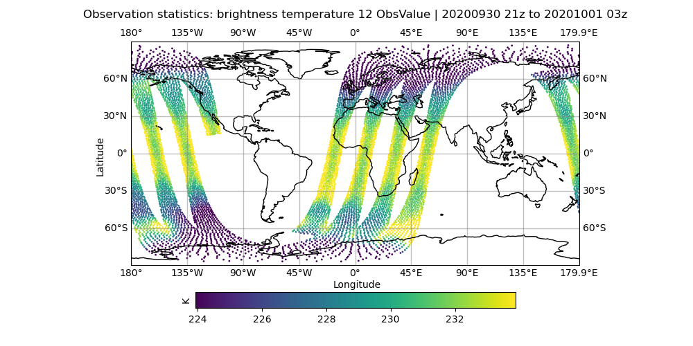
# Let's look at the brightness_temperature variable for channel 12 in the AMSU-A, NOAA19 data

# input observations
# Use your favorite editor to edit the configuration files
# Examples below are for the 'vi' editor
vi Diagnostics/hofx_map.yaml
  # change the hofx files entry to "amsua_n19_3denvar_2020100100_*.nc4"
  # change the variable spec to brightness_temperature_12@ObsValue
  # make sure colorbar min and max controls are commented out
fv3jeditools.x 2020-10-01T00:00:00 Diagnostics/hofx_map.yaml

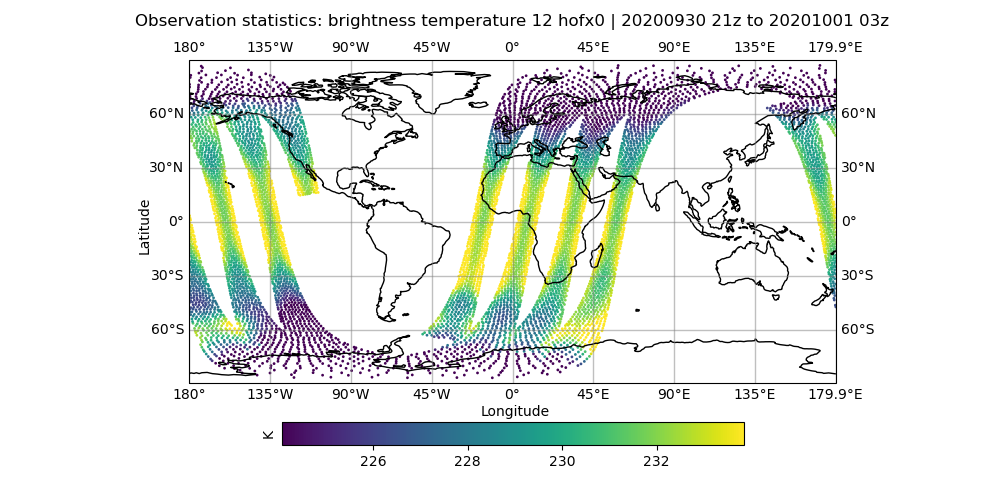
# initial hofx result
vi Diagnostics/hofx_map.yaml
  # change the variable spec to brightness_temperature_12@hofx0
  # make sure colorbar min and max controls are commented out
fv3jeditools.x 2020-10-01T00:00:00 Diagnostics/hofx_map.yaml

# obs minus background
vi Diagnostics/hofx_map.yaml
  # change the variable to brightness_temperature_12@ombg
  # make sure colorbar min and max controls are set to -/+1
fv3jeditools.x 2020-10-01T00:00:00 Diagnostics/hofx_map.yaml

# obs minus analysis
vi Diagnostics/hofx_map.yaml
  # change the variable to brightness_temperature_12@oman
  # make sure colorbar min and max controls are set to -/+1
fv3jeditools.x 2020-10-01T00:00:00 Diagnostics/hofx_map.yaml

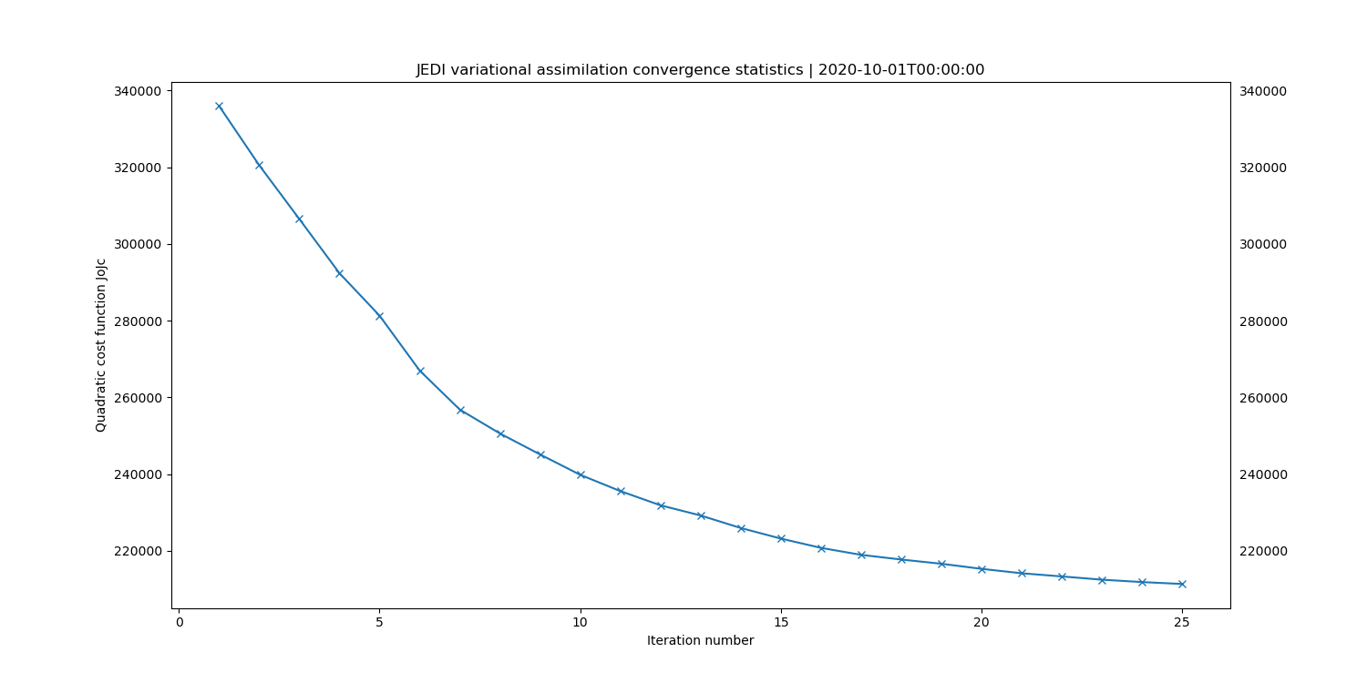
# cost function convergence
fv3jeditools.x 2020-10-01T00:00:00 Diagnostics/da_convergence.yaml

# innovations
vi Diagnostics/hofx_innovations.yaml
  # change the hofx files entry to "amsua_n19_3denvar_2020100100_*.nc4"
  # change variable to brightness_temperature_12
  # make sure "number of outer loops" is set to 1 since we ran with one outer loop
  # set the "number of bins" spec to 70
  #     the number of bins controls how many histogram bins are created
  #     the satellite obs in this run have fairly low obs counts (for runtime sake)
  #     so the number of bins needs to be around 70 to mitigate noise in the plot
fv3jeditools.x 2020-10-01T00:00:00 Diagnostics/hofx_innovations.yaml

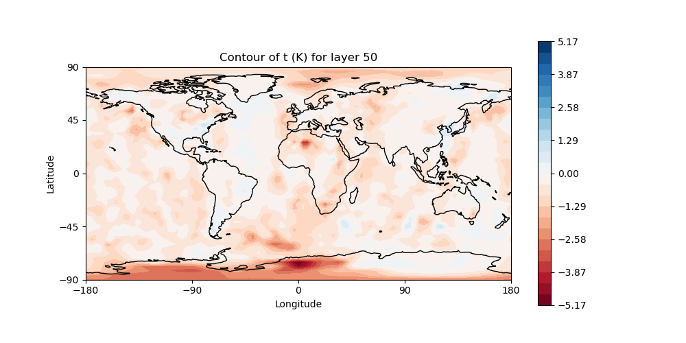
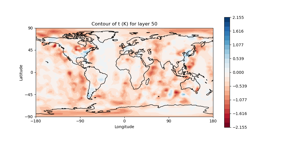
# Plot temperature increment on level 50
# Make sure "field name" is set to "t" and "model layer" is set to 50
# in the configuration file: Diagnostics/field_plot.yaml
fv3jeditools.x 2020-10-01T00:00:00 Diagnostics/field_plot.yaml

Create a subdirectory called “Run_Orig” and move any plots from yesterday’s exercise into this subdirectory.

# Save the plots from the original run
cd ~/jedi/tutorials/20201001_0000z
mkdir Run_Orig
mv Logs/*.png Run_Orig
mv Data/hofx/*.png Run_Orig
mv Data/increment/*.png Run_Orig

Compare the AMSU-A, NOAA19 input observations with the initial H(x), which are the simulated observations from the model fields. The general patterns should be similar, but note that the finer details don’t exactly match. The innovation plots show the differences between the simulated observations, H(x), and the actual observations in a PDF style.

Take note of how many observations were assimilated. This information is in the log file for the 3DVar run and a quick way to look at this is to grep out the lines containing Jo cost function information. Running the following command:

grep CostJo Logs/3denvar.log > Jo.stats

should yield a filed called “Jo.stats” that contains lines like the following:

Test     : CostJo   : Nonlinear Jo(Aircraft) = 238308, nobs = 268090, Jo/n = 0.88891, err = 2.19395
Test     : CostJo   : Nonlinear Jo(AMSUA-NOAA19) = 53002.4, nobs = 60049, Jo/n = 0.882653, err = 2.00229
Test     : CostJo   : Nonlinear Jo(Aircraft) = 159577, nobs = 268045, Jo/n = 0.595338, err = 2.19395
Test     : CostJo   : Nonlinear Jo(AMSUA-NOAA19) = 22047.7, nobs = 60049, Jo/n = 0.367162, err = 2.00229

Note that this sample shows one outer loop with 2 observation types (Aircraft, AMSUA-NOAA19). The first two lines are before the output loop starts, and the last two lines after the outer loop completes. The nobs = entries reveal the number of observations assimilated (after QC filtering) and the Jo/n = entries show whether the process is converging (ie, the numbers corresponding to each observation type should be decreasing).

Move the Jo.stats file into the “Run_Orig” subdirectory aside the plots.

Step 2: Add a new ObsSpace to the 3DVar configuration

The ObsSpace declarations are located near the middle of the the YAML configuration file under a section called observations Here is an excerpt from the YAML configuration corresponding to the results shown in the previous step (file: ~/jedi/tutorials/20201001_0000z/Config/3denvar.yaml):

cost function:
...
  # Observations to assimilate
  # --------------------------
  observations:

  # Aircraft
  - obs space:
      name: Aircraft
      ...

  # AMSU-A NOAA19
  - obs space:
      name: AMSUA-NOAA19
      obsdatain:
        obsfile: Data/obs/amsua_n19_obs_2020100100.nc4
      obsdataout:
        obsfile: Data/hofx/amsua_n19_3denvar_2020100100.nc4
      simulated variables: [brightness_temperature]
      channels: 4-6,9-14
    obs operator:
      name: CRTM
      Absorbers: [H2O,O3]
#     Clouds: [Water, Ice]
#     Cloud_Fraction: 1.0
      obs options:
        Sensor_ID: amsua_n19
        EndianType: little_endian
        CoefficientPath: Data/crtm/
    obs error:
      covariance model: diagonal
    ...

For brevity’s sake, only the details under the AMSUA-NOAA19 - obs space are shown. There exist two - obs space: sections corresponding to the two observation types in the Jo stats from the previous section. Let’s add another radiance type, the AMSUA instrument on the AQUA satellite, to the mix. Look at the AMSUA-NOAA19 - obs space definition above, and note the path to the input observation file given by the obsfile keyword in the obsdatain section. Do a directory listing in the directory where AMSUA file resides:

ls -1 ~/jedi/tutorials/20201001_0000z/Data/obs

which should yield a list like:

aircraft_obs_2020100100.nc4
airs_aqua_obs_2020100100.nc4
amsua_aqua_obs_2020100100.nc4
amsua_metop-a_obs_2020100100.nc4
amsua_metop-b_obs_2020100100.nc4
amsua_n15_obs_2020100100.nc4
amsua_n18_obs_2020100100.nc4
amsua_n19_obs_2020100100.nc4
atms_n20_obs_2020100100.nc4
atms_npp_obs_2020100100.nc4
...

The AMSUA-AQUA observation file is: amsua_aqua_obs_2020100100.nc4.

Let’s start by copy-and-pasting the AMSUA-NOAA19 spec in the YAML file (~/jedi/tutorials/20201001_0000z/Config/3denvar.yaml). Don’t worry about the obs filters section yet, so just copy-and-paste the - obs space, obs operator and obs error sections. Note that you want to paste after the end of the AMSUA-NOAA19 spec in the YAML, meaning that you insert the copy after the obs filters section under the AMSUA-NOAA19 - obs space specification.

Here is what you copy:

# AMSU-A NOAA19
- obs space:
    name: AMSUA-NOAA19
    obsdatain:
      obsfile: Data/obs/amsua_n19_obs_2020100100.nc4
    obsdataout:
      obsfile: Data/hofx/amsua_n19_3denvar_2020100100.nc4
    simulated variables: [brightness_temperature]
    channels: 4-6,9-14
  obs operator:
    name: CRTM
    Absorbers: [H2O,O3]
#     Clouds: [Water, Ice]
#     Cloud_Fraction: 1.0
    obs options:
      Sensor_ID: amsua_n19
      EndianType: little_endian
      CoefficientPath: Data/crtm/
  obs error:
    covariance model: diagonal

And here is where to paste. Note the use of “…” to mark where details have been left out in this listing for brevity’s sake. The paste should occur where marked with “<— Insert copy here”.

observations:

...

# AMSU-A NOAA19
- obs space:
    name: AMSUA-NOAA19
    ...
  obs operator:
    name: CRTM
    ...
  obs error:
    covariance model: diagonal
  obs filters:
  - filter: Bounds Check
    filter variables:
    - name: brightness_temperature
      channels: 4-6,9-14
    minvalue: 100.0
    maxvalue: 500.0
  - filter: Background Check
    filter variables:
    - name: brightness_temperature
      channels: 4-6,9-14
    threshold: 3.0
  - filter: Domain Check
    filter variables:
    - name: brightness_temperature
      channels: 4-6,9-14
    where:
    - variable:
        name: scan_position@MetaData
      minvalue: 4
      maxvalue: 27
    - variable:
        name: brightness_temperature_1@ObsValue
      minvalue: 50.0
      maxvalue: 550.0
    - variable:
        name: brightness_temperature_2@ObsValue
      minvalue: 50.0
      maxvalue: 550.0
    - variable:
        name: brightness_temperature_3@ObsValue
      minvalue: 50.0
      maxvalue: 550.0
    - variable:
        name: brightness_temperature_4@ObsValue
      minvalue: 50.0
      maxvalue: 550.0
    - variable:
        name: brightness_temperature_6@ObsValue
      minvalue: 50.0
      maxvalue: 550.0
    - variable:
        name: brightness_temperature_15@ObsValue
      minvalue: 50.0
      maxvalue: 550.0

                                   <----------- Insert copy here

# Diagnostics to write
final:
  diagnostics:
    departures: oman
...

After pasting, take note of the indentation and make sure it is correct. For example if you copy-and-pasted from the activity instructions instead of the yaml file, then the indentation will be off since the activity instructions left-justified the yaml contents.

For the sample AMSUA-AQUA observation file, let’s assimilate channels 3 and 6 through 15. The CRTM identifier for the AMSUA instrument on the AQUA platform is “amsua_aqua”. This should be enough information to change the copy-and-pasted - obs space spec into one for AMSUA-AQUA.

In the CostJo listings we took a look at earlier, the ObsSpace name is used to formulate the Jo stats message so make sure to update that name for AMSUA-AQUA. Also, don’t forget to change the obsdataout file so we don’t overwrite the AMSUA-NOAA19 hofx data.

As a hint, you should be making changes for the name keyword under - obs space, both obsfile keywords under obsdatain and obsdataout, the channels keyword under - obs space, and the Sensor_ID keyword under obs options.

We should be ready to try the assimilation run now.

Step 3: Run the 3DVar job (including the AMSUA-AQUA observations)

Make sure you are in the proper directory, and re-run the 3DVar and increment jobs.

cd ~/jedi/tutorials/20201001_0000z

# run the 3DVar assimilation
mpirun -np 6 $JEDIBUILD/bin/fv3jedi_var.x Config/3denvar.yaml Logs/3denvar.log

# create the increment
mpirun -np 6 $JEDIBUILD/bin/fv3jedi_diffstates.x Config/create_increment_3denvar.yaml

Generate the plots as before and the Jo.stats file. When making the hofx and innovation plots, use the amsua, aqua (instead of n19) data files so you can later see the changes after the next step. The Jo.stats file should look like this:

Test     : CostJo   : Nonlinear Jo(Aircraft) = 238308, nobs = 268090, Jo/n = 0.88891, err = 2.19395
Test     : CostJo   : Nonlinear Jo(AMSUA-NOAA19) = 53002.4, nobs = 60049, Jo/n = 0.882653, err = 2.00229
Test     : CostJo   : Nonlinear Jo(AMSUA-AQUA) = 375629, nobs = 89837, Jo/n = 4.18123, err = 2.37315
Test     : CostJo   : Nonlinear Jo(Aircraft) = 160750, nobs = 268044, Jo/n = 0.599716, err = 2.19397
Test     : CostJo   : Nonlinear Jo(AMSUA-NOAA19) = 22532.3, nobs = 60049, Jo/n = 0.375232, err = 2.00229
Test     : CostJo   : Nonlinear Jo(AMSUA-AQUA) = 233847, nobs = 89837, Jo/n = 2.60301, err = 2.37315

Note the additional lines indicating the inclusion of the AMSUA-AQUA observations in the assimilation.

Create another subdirectory, “Run_1”, and store the plots and Jo.stats file there. Take a look at the plots paying attention to the changes in the increment and convergence plots.

Step 4: Add filtering for AMSUA-AQUA observations

Cut-and-paste the obs filters section from the AMSUA-NOAA19 - obs space into the AMSUA-AQUA - obs space configuration (Config/3denvar.yaml):

obs filters:
- filter: Bounds Check
  filter variables:
  - name: brightness_temperature
    channels: 4-6,9-14
  minvalue: 100.0
  maxvalue: 500.0
- filter: Background Check
  filter variables:
  - name: brightness_temperature
    channels: 4-6,9-14
  threshold: 3.0
- filter: Domain Check
  filter variables:
  - name: brightness_temperature
    channels: 4-6,9-14
  where:
  - variable:
      name: scan_position@MetaData
    minvalue: 4
    maxvalue: 27
  - variable:
      name: brightness_temperature_1@ObsValue
    minvalue: 50.0
    maxvalue: 550.0
  - variable:
      name: brightness_temperature_2@ObsValue
    minvalue: 50.0
    maxvalue: 550.0
  - variable:
      name: brightness_temperature_3@ObsValue
    minvalue: 50.0
    maxvalue: 550.0
  - variable:
      name: brightness_temperature_4@ObsValue
    minvalue: 50.0
    maxvalue: 550.0
  - variable:
      name: brightness_temperature_6@ObsValue
    minvalue: 50.0
    maxvalue: 550.0
  - variable:
      name: brightness_temperature_15@ObsValue
    minvalue: 50.0
    maxvalue: 550.0

This section is okay as is, except for the channel selection. Change the three channels keywords to match the channel selection under the filter variables keyword (in the AMSUA-AQUA - obs space spec).

Re-run the 3Dvar and increment jobs, generate the Jo.stats file and take a look at the Jo.stats file. You should see messages indicating that zero obs were assimilated from the new AMSUA-AQUA data similar to these:

Test     : CostJo   : Nonlinear Jo(Aircraft) = 238308, nobs = 268090, Jo/n = 0.88891, err = 2.19395
Test     : CostJo   : Nonlinear Jo(AMSUA-NOAA19) = 53002.4, nobs = 60049, Jo/n = 0.882653, err = 2.00229
Test     : CostJo   : Nonlinear Jo(AMSUA-AQUA) = 0 --- No Observations
CostJo: No Observations!!!
Test     : CostJo   : Nonlinear Jo(Aircraft) = 159577, nobs = 268045, Jo/n = 0.595338, err = 2.19395
Test     : CostJo   : Nonlinear Jo(AMSUA-NOAA19) = 22047.7, nobs = 60049, Jo/n = 0.367162, err = 2.00229
Test     : CostJo   : Nonlinear Jo(AMSUA-AQUA) = 0 --- No Observations
CostJo: No Observations!!!

At this point, you would start a debug process to find out why no AMSUA-AQUA observations are being used. For the sake of brevity, the answer in this case is that channels 1, 2, and 4 contain missing data for all locations of the brightness temperature ObsValue variables in the input obs file. This is causing the filter to strip out all observations due to the specs under the where keyword. The fix is to remove the sections for the variabes brightness_temperature1@Obsvalue, brightness_temperature_2@ObsValue and brightness_temperature_4@ObsValue under the where keyword.

Make these changes to the config file, re-run the assimilation, regenerate the Jo.stats file and check to make sure observations from AMSUA-AQUA are being assimilated. Your Jo.stats files should look similar to this:

Test     : CostJo   : Nonlinear Jo(Aircraft) = 238308, nobs = 268090, Jo/n = 0.88891, err = 2.19395
Test     : CostJo   : Nonlinear Jo(AMSUA-NOAA19) = 53002.4, nobs = 60049, Jo/n = 0.882653, err = 2.00229
Test     : CostJo   : Nonlinear Jo(AMSUA-AQUA) = 60097.2, nobs = 71091, Jo/n = 0.845356, err = 2.4969
Test     : CostJo   : Nonlinear Jo(Aircraft) = 159856, nobs = 268047, Jo/n = 0.596374, err = 2.19396
Test     : CostJo   : Nonlinear Jo(AMSUA-NOAA19) = 22141, nobs = 60049, Jo/n = 0.368716, err = 2.00229
Test     : CostJo   : Nonlinear Jo(AMSUA-AQUA) = 28407.8, nobs = 71091, Jo/n = 0.399598, err = 2.4969

Note that fewer obs for AMSUA-AQUA are being assimilated compared to Run_1.

When you’ve confirmed that AMSUA-AQUA obs are being assimilated, generate the plots as before. Create another subdirectory, “Run_2”, and move the Jo.stats file and plots into that subdirectory. Take a look at the Run_2 plots, again paying attention to the increment and convergence plots. Note the differences in the increment that adding AMSUA-AQUA obs made (Run_Orig vs Run_1), and the differences in the increment that the filtering of the AMSUA-AQUA obs made (Run_1 vs Run_2).

Sample plots

Here are some sample plots for this exercise. These plots were generated using the original (Tuesday A) configuration, and the changes from today’s exercise. If you made changes to the configuration (eg, added more iterations), then your results may not exactly match what is show below, but they should still be generally the same.

Input Observations

AMSU-A, NOAA19 Observations

AMSU-A, AQUA Observations

Original Run

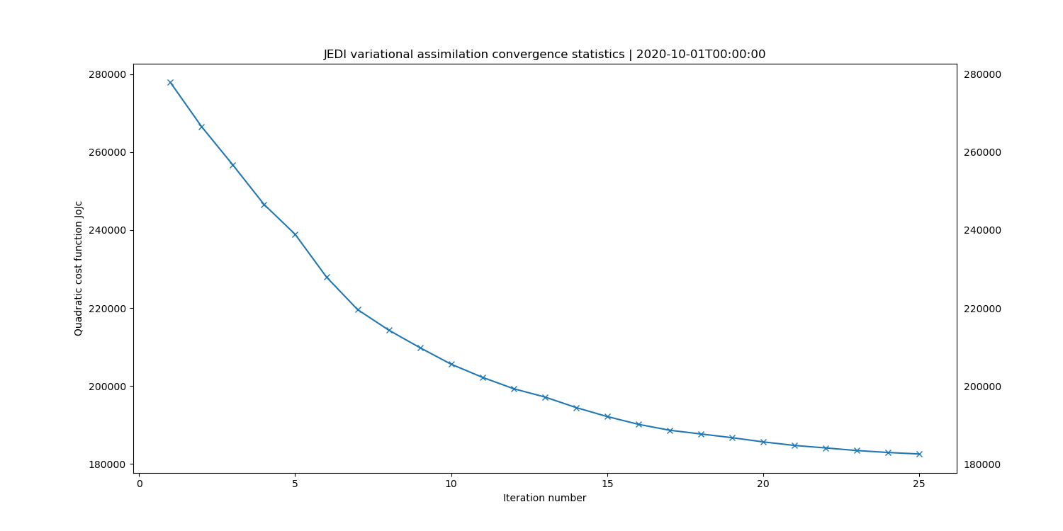
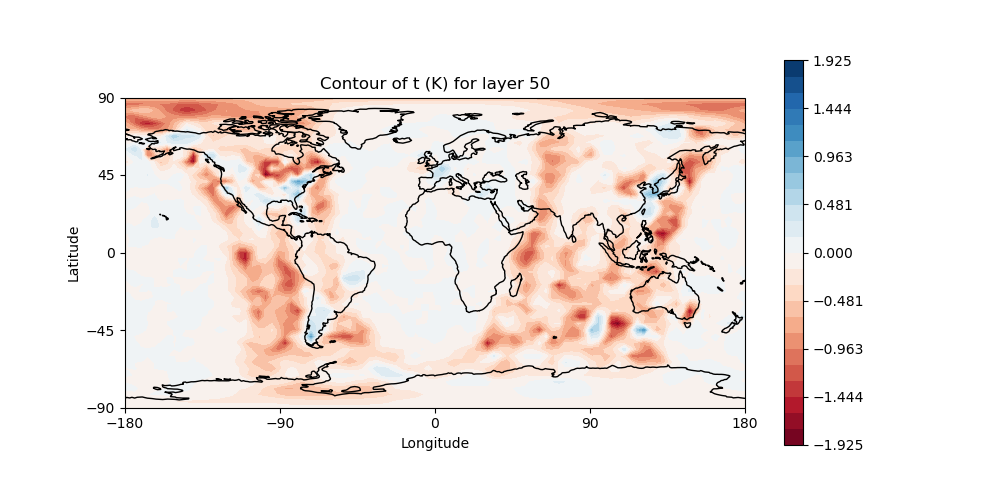
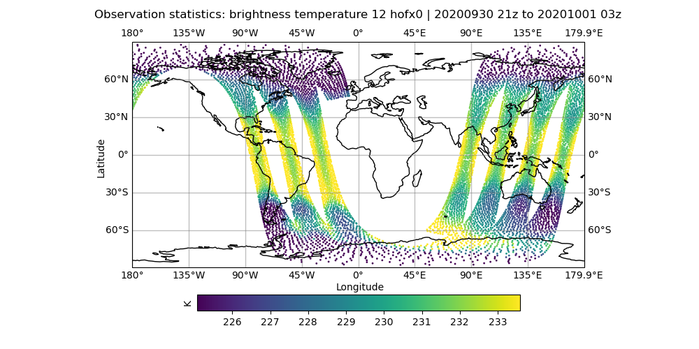
left: JoJc convergence, center: increment of T, right: AMSU-A, NOAA19 initial H(x)

(click on image to magnify)

Run_1

left: JoJc convergence, center: increment of T, right: AMSU-A, AQUA initial H(x)

Run_2

left: JoJc convergence, center: increment of T, right: AMSU-A, AQUA initial H(x)