Tuesday A: Adding new observations to be assimilated
Introduction:
In this activity we will take a look at adding new observations into yesterday’s 3DVar exercise. This task typically involves the following steps:
- Convert your raw observation file into a IODA formatted observation file.
- Add a new ObsSpace definition to the YAML configuration file for the 3DVar run.
These tasks can involve some software development depending on whether your new observation type can be handled by existing IODA file converter programs and UFO obs operators. For today’s exercise, we will use existing IODA observation files and UFO obs operators, reducing your task to simply editing the 3DVar YAML configuration file.
The goal of this exercise is to learn how to manage the assimlation of different sets of observations in the JEDI system.
Step 1: Save results from yesterday
We are going to add the new observation type, regenerate the results and then compare the new results to yesterday’s results. Create a subdirectory called “Day1” and move any plots from yesterday’s exercise into this subdirectory. There are a couple of plots that will be helpful for today’s exercise so let’s make sure these have been generated:
# Save yesterday's plots
cd ~/academy/run-hyb-3dvar
mkdir Day1
mv *.png Day1

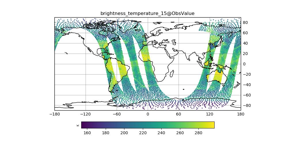
# Input amsua, metop-a observations, channel 15
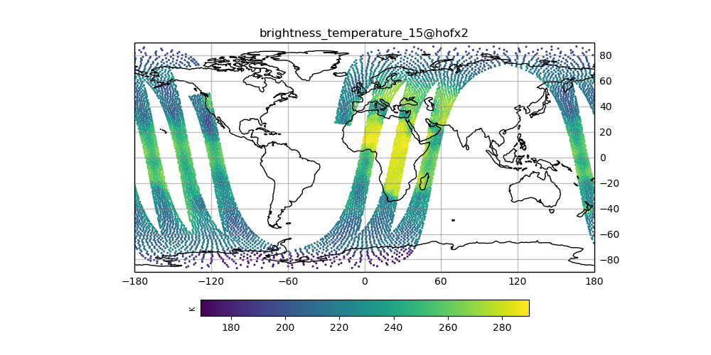
hofx.py -f hofx/amsua_metop-a_hyb-3dvar-gfs_2018041500_m_NPROC.nc4 -v brightness_temperature_15@ObsValue

# amsua, metop-a H(x) at end of the run, channel 15
hofx.py -f hofx/amsua_metop-a_hyb-3dvar-gfs_2018041500_m_NPROC.nc4 -v brightness_temperature_15@hofx2

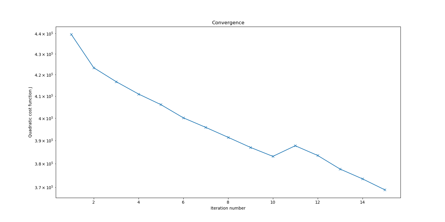
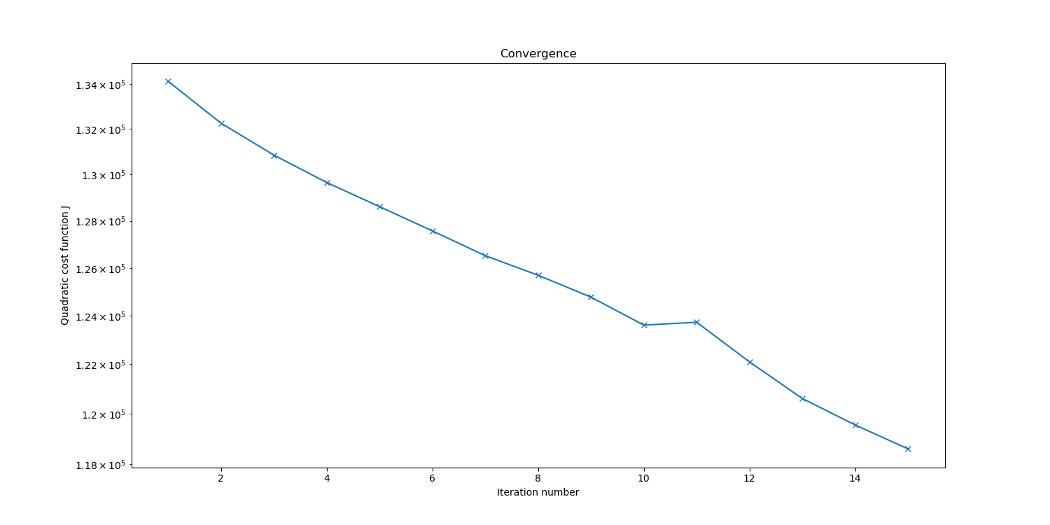
# Convergence of J cost function
convergence.py -l logs/hyb-3dvar.log -j J

# Innovation (departure) of asmua, metop-a, channel 15
innovation.py -f hofx/amsua_metop-a_hyb-3dvar-gfs_2018041500_m_NPROC.nc4 -v brightness_temperature_15 -n 2

# Increment of temperature at model level 5
field_level_plot.py -i increment/hyb-3dvar-gfs.20180415_000000.nc4 -l 5 -f T

# Save these plots
mkdir Day2_Run1
mv *.png Day2_Run1
Compare the amsu-a, metop-a input observations with the final H(x), which are the simulated observations from the model fields. The general patterns should be similar, but note that the finer details don’t exactly match. The innovation plots show the differences between the simulated observations, H(x), and the actual observations.
Take note of how many observations were assimilated. This information is in the log file for the 3DVar run and a quick way to look at this is to grep out the lines containing Jo cost function information. Running the following command:
grep CostJo logs/hyb-3dvar.log > Jo.stats
should yield a filed called “Jo.stats” that contains lines like the following:
Test     : CostJo   : Nonlinear Jo(Aircraft) = 2883.51, nobs = 1439, Jo/n = 2.00383, err = 2.67702
Test     : CostJo   : Nonlinear Jo(Radiosonde) = 2124.55, nobs = 1131, Jo/n = 1.87847, err = 2.0616
Test     : CostJo   : Nonlinear Jo(GnssroRef) = 0 --- No Observations
CostJo: No Observations!!!
Test     : CostJo   : Nonlinear Jo(AMSUA-METOPA) = 59339.9, nobs = 53349, Jo/n = 1.1123, err = 1.77314
Note that this sample shows one iteration with 4 observation types (Aircraft, Radiosonde, GnssroRef, AMSUA-METOPA).
The nobs = entries reveal the number of observations assimilated (after QC filtering) and the Jo/n = entries show whether the process is converging (ie, the numbers corresponding to each observation type should be decreasing).
The GnssroRef (RO refractivity) line has a message indicating that no observations were assimilated during this iteration.
Further investigation in the log file reveals the following lines:
BackgroundCheck obserr: GnssroRef refractivity nlocs = 20, nobs= 20 Min=0.0111865, Max=3.5151
processing a float: 3
processWhere: selected 0 obs.
...
QC GnssroRef refractivity: 20 removed by thinning.
QC GnssroRef refractivity: 0 passed out of 20 observations.
which indicate that the filtering operations on the GnssroRef removed all of the observations from the input file.
Move the Jo.stats file into the “Day2_Run1” subdirectory aside the plots.
Step 2: Add a new ObsSpace to the 3DVar configuration
The ObsSpace declarations are located in the ObsTypes section under the Jo section in the YAML configuration file. Here is the YAML configuration corresponding to the results shown in the previous step (file: ~/academy/conf/hyb-3dvar.yaml):
Jo:
  ObsTypes:
  - ObsSpace:
      name: Aircraft
    ...
  - ObsSpace:
      name: Radiosonde
    ...
  - ObsSpace:
      name: GnssroRef
    ...
  - ObsSpace:
      name: AMSUA-METOPA
      ObsDataIn:
        obsfile: data/obs/amsua_metop-a_obs_2018041500.nc4
      ObsDataOut:
        obsfile: run-hyb-3dvar/hofx/amsua_metop-a_hyb-3dvar-gfs_2018041500_m.nc4
      simulate:
        variables: [brightness_temperature]
        channels: 1-6,9-11,15
    ObsOperator:
      name: CRTM
      Absorbers: [H2O,O3]
      ObsOptions:
        Sensor_ID: amsua_metop-a
        EndianType: little_endian
        CoefficientPath: /Users/steveherbener/projects/fv3-bundle/build/fv3-jedi/test/Data/crtm/
    Covariance:
      covariance: diagonal
    ObsFilters:
    - Filter: Bounds Check
      filter variables:
      - name: brightness_temperature
        channels: 1-6,9-11,15
      minvalue: 100.0
      maxvalue: 500.0
    - Filter: Background Check
      filter variables:
      - name: brightness_temperature
        channels: 1-6,9-11,15
      threshold: 3.0
For brevity’s sake, only the details under the AMSU-A, METOP-A ObsSpace are shown.
There exist four - ObsSpace: sections corresponding to the four observation types in the Jo stats from the previous section.
Let’s add another radiance type, the AMSUA instrument on the AQUA satellite, to the mix.
Look at the AMSUA-METOPA ObsSpace definition above, and note the path to the input observation file given by the obsfile keyword in the ObsDataIn section.
Do a directory listing in the directory where AMSUA file resides:
ls ~/academy/data/obs
which should yield a list like:
amsua_aqua_obs_2018041500.nc4         amsua_metop-b_obs_2018041500.nc4
amsua_metop-a_obs_2018041500.nc4      amsua_n15_obs_2018041500.nc4
The AMSUA-AQUA observation file is: amsua_aqua_obs_2018041500_m.nc4.
Let’s start by cut-and-pasting the AMSUA-METOPA spec in the YAML file (~/academy/conf/hyb-3dvar.yaml). Don’t worry about the ObsFilter section yet, so just cut-and-paste the ObsSpace, ObsOperator and Covariance sections:
- ObsSpace:
    name: AMSUA-METOPA
    ObsDataIn:
      obsfile: data/obs/amsua_metop-a_obs_2018041500.nc4
    ObsDataOut:
      obsfile: run-hyb-3dvar/hofx/amsua_metop-a_hyb-3dvar-gfs_2018041500_m.nc4
    simulate:
      variables: [brightness_temperature]
      channels: 1-6,9-11,15
  ObsOperator:
    name: CRTM
    Absorbers: [H2O,O3]
    ObsOptions:
      Sensor_ID: amsua_metop-a
      EndianType: little_endian
      CoefficientPath: /Users/steveherbener/projects/fv3-bundle/build/fv3-jedi/test/Data/crtm/
  Covariance:
    covariance: diagonal
For the sample AMSUA, AQUA observation file, let’s assimilate channels 3 and 6 through 15. The CRTM identifier for the AMSUA instrument on the AQUA platform is “amsua_aqua”. This should be enough information to change the cut-and-pasted ObsSpace spec into one for AMSUA-AQUA.
In the CostJo listings we took a look at earlier, the ObsSpace name is used to formulate the Jo stats message so make sure to update that name for amsua, aqua. Also, don’t forget to change the ObsDataOut file so we don’t overwrite the AMSUA, METOPA hofx data.
As a hint, you should be making changes for the name keyword under ObsSpace, both obsfile keywords under ObsDataIn and ObsDataOut, the channels keyword under simulate, and the Sensor_ID keyword under ObsOptions.
We should be ready to try the assimilation run now.
Step 3: Run the 3DVar job (including the amsua-aqua observations)
Make sure you are in the proper directory, and re-run the 3DVar job.
cd ~/academy
./run.bash hyb-3dvar
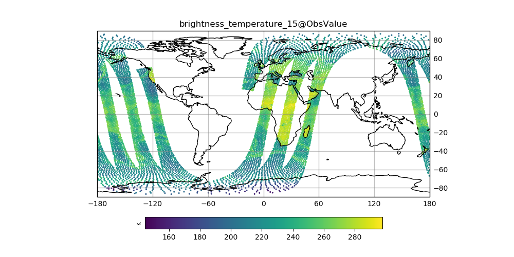
Generate the plots as before and the Jo.stats file. When making the hofx and innovation plots, use the amsua, aqua (instead of metop-a) data so you can later see the changes after the next step.
Create another subdirectory, “Day2_Run2”, and store the plots and Jo.stats file there. Take a look at the plots paying attention to the changes in the increment and convergence plots.
Step 4: Add filtering for amsua-aqua observations
Cut-and-paste the ObsFilter section from the AMSUA-METOPA ObsSpace into the AMSUA-AQUA ObsSpace configuration (conf/hyb-3dvar.yaml):
ObsFilters:
- Filter: Bounds Check
  filter variables:
  - name: brightness_temperature
    channels: 1-6,9-11,15
  minvalue: 100.0
  maxvalue: 500.0
- Filter: Background Check
  filter variables:
  - name: brightness_temperature
    channels: 1-6,9-11,15
  threshold: 3.0
This section is okay as is, except for the channel selection.
Change the two channels keywords to match the channel selection under the simulate keyword (in the amsua, aqua ObsSpace spec).
Re-run the 3Dvar and generate the Jo.stats file and plots. Create another subdirectory, “Day2_Run3”, and move the Jo.stats file and plots into that subdirectory. Take a look at the Day2_Run3 plots, again paying attention to the increment and convergence plots.
Sample plots
Here are some sample plots for this exercise. These plots were generated using the original (Day1) configuration, and the changes from today’s exercise. If you made changes to the configuration (eg, added more iterations), then your results may not exactly match what is show below, but they should still be generally the same.
Original Run
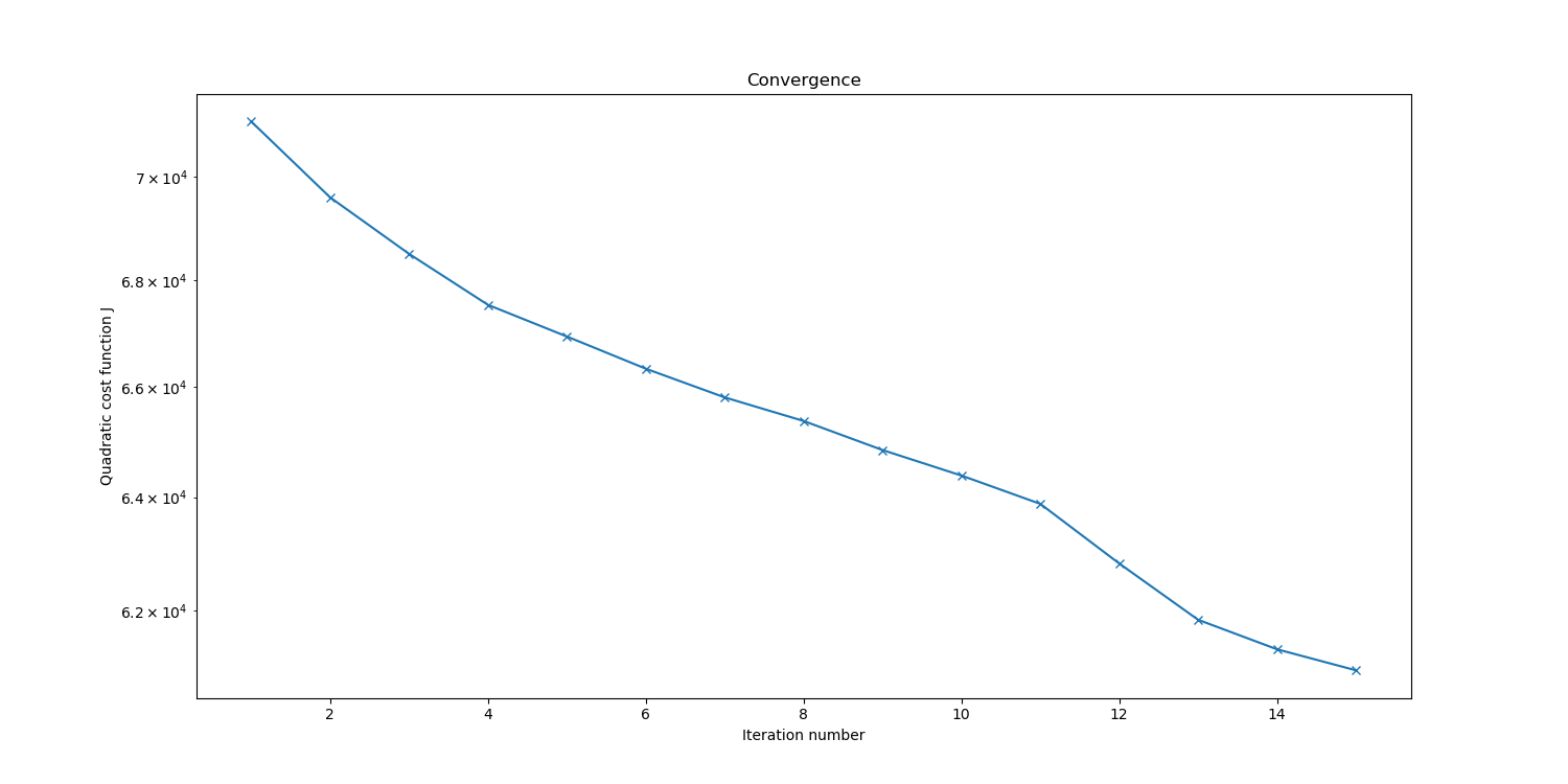
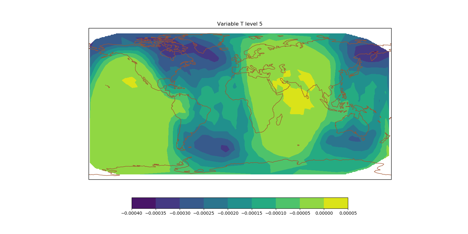

left: J convergence, center: increment of T, right: AMSU-A, METOP-A final H(x)
(click on image to magnify)
